Python Data Science Series Part 1: NumPy Foundations

The Evolution of NumPy

Historical Context

NumPy's story begins in the mid-1990s when Python was emerging as a scientific computing platform:

• 1995: Jim Hugunin creates Numeric, the first array package for Python
• 2001: Numarray emerges to address Numeric's limitations with large arrays
• 2005: Travis Oliphant unifies Numeric and Numarray into NumPy, combining the best of both
• 2006-Present: NumPy becomes the de facto standard for numerical computing in Python

Why It Matters Today

NumPy's importance has only grown with the data science revolution:

• Foundation for ML: Deep learning frameworks like TensorFlow and PyTorch use NumPy-compatible tensors
• Data pipelines: Pandas DataFrames are built on NumPy arrays underneath
• Scientific computing: SciPy extends NumPy for advanced scientific functions
• Industry standard: Over 1,000 packages depend on NumPy in the Python ecosystem

NumPy Fundamentals

Installation and Setup

Installing NumPy is straightforward with pip:

# Install NumPy
pip install numpy

# Verify installation
python -c "import numpy as np; print(f'NumPy version: {np.__version__}')"

The ndarray: NumPy's Core Data Structure

The ndarray (N-dimensional array) is NumPy's fundamental object. Unlike Python lists, ndarrays:

• Store elements of the same type (homogeneous)
• Use contiguous memory for fast access
• Support vectorized operations without explicit loops
• Enable broadcasting for efficient element-wise operations

import numpy as np

# Creating arrays from Python lists
arr_1d = np.array([1, 2, 3, 4, 5])
arr_2d = np.array([[1, 2, 3], [4, 5, 6]])

print("1D array:", arr_1d)
print("Shape:", arr_1d.shape)  # (5,)
print("2D array:\n", arr_2d)
print("Shape:", arr_2d.shape)  # (2, 3)

Working with Arrays

Array Creation Methods

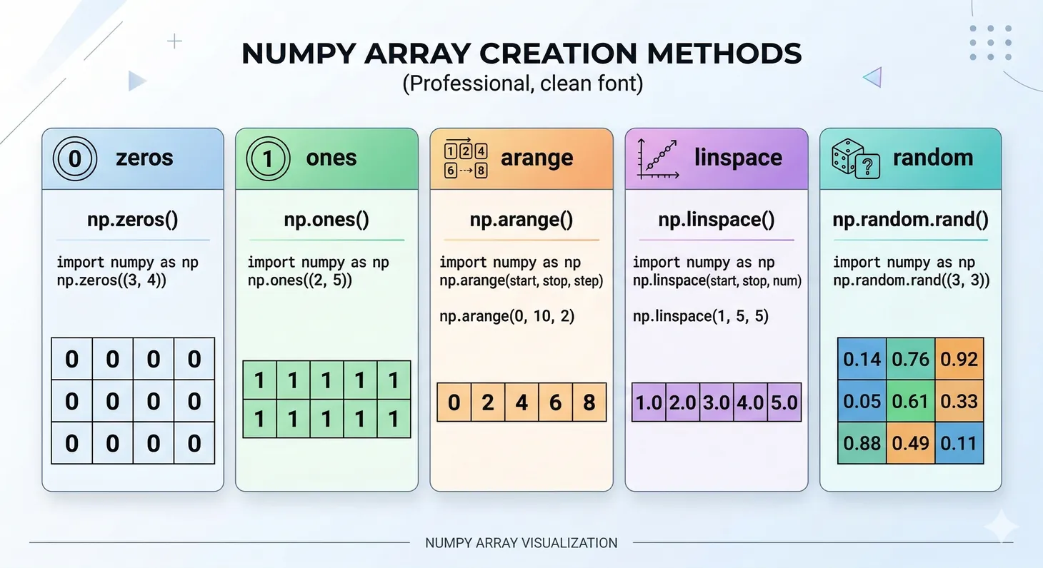
NumPy provides numerous ways to create arrays beyond converting lists:

import numpy as np

# np.zeros(shape, dtype=float) - Create array filled with zeros
# Parameters:
#   shape: int or tuple - Dimensions (e.g., 3 for 1D, (3,4) for 2D)
#   dtype: data type - Type of elements (default: float64)
zeros = np.zeros((3, 4))        # 3x4 array of zeros (floats)
print("Zeros:\n", zeros)

# np.ones(shape, dtype=float) - Create array filled with ones
# Parameters same as zeros
ones = np.ones((2, 3))          # 2x3 array of ones (floats)
print("Ones:\n", ones)

# np.empty(shape, dtype=float) - Create uninitialized array (faster but random values)
# Use only when you'll immediately fill all values
empty = np.empty((2, 2))        # Uninitialized 2x2 array
print("Empty (random values):\n", empty)

import numpy as np

# np.arange([start,] stop[, step,], dtype=None) - Create range of values
# Parameters:
#   start: number - Starting value (inclusive, default: 0)
#   stop: number - Ending value (exclusive)
#   step: number - Spacing between values (default: 1)
#   dtype: data type - Type of elements (inferred if not specified)
range_arr = np.arange(0, 10, 2)       # [0, 2, 4, 6, 8] - start=0, stop=10, step=2
print("Range:", range_arr)

# np.linspace(start, stop, num=50, endpoint=True) - Evenly spaced values
# Parameters:
#   start: number - Starting value (inclusive)
#   stop: number - Ending value (inclusive if endpoint=True)
#   num: int - Number of samples to generate (default: 50)
#   endpoint: bool - Include stop value (default: True)
linspace = np.linspace(0, 1, 5)       # 5 evenly spaced: [0, 0.25, 0.5, 0.75, 1]
print("Linspace:", linspace)

# Key difference: arange uses step size, linspace uses number of points

import numpy as np

# np.eye(N, M=None, k=0, dtype=float) - Create identity or diagonal matrix
# Parameters:
#   N: int - Number of rows
#   M: int - Number of columns (default: same as N for square matrix)
#   k: int - Index of diagonal (0=main, 1=above, -1=below)
#   dtype: data type - Type of elements
identity = np.eye(3)                   # 3x3 identity matrix (1s on diagonal, 0s elsewhere)
print("Identity:\n", identity)

# np.diag(v, k=0) - Extract diagonal or create diagonal matrix
# Parameters:
#   v: array - 1D array to place on diagonal, or 2D array to extract diagonal from
#   k: int - Diagonal offset (0=main, 1=above, -1=below)
diagonal = np.diag([1, 2, 3, 4])      # Create diagonal matrix from 1D array
print("Diagonal:\n", diagonal)

# Extract diagonal from 2D array
matrix = np.array([[1, 2, 3], [4, 5, 6], [7, 8, 9]])
diag_values = np.diag(matrix)          # Extract [1, 5, 9]
print("Extracted diagonal:", diag_values)

Array Attributes

Understanding array properties is essential for effective NumPy usage:

import numpy as np

arr = np.array([[1, 2, 3], [4, 5, 6]])

print("Shape:", arr.shape)           # (2, 3) - dimensions
print("Size:", arr.size)             # 6 - total elements
print("Dtype:", arr.dtype)           # int64 - data type
print("Ndim:", arr.ndim)             # 2 - number of dimensions
print("Itemsize:", arr.itemsize)     # 8 - bytes per element

# Same data, different memory footprints
arr_int64 = np.array([1, 2, 3], dtype=np.int64)
arr_int8 = np.array([1, 2, 3], dtype=np.int8)

print(f"int64 uses: {arr_int64.nbytes} bytes")  # 24 bytes
print(f"int8 uses: {arr_int8.nbytes} bytes")    # 3 bytes

Array Operations & Vectorization

Vectorization: The NumPy Advantage

Vectorization means operations apply to entire arrays without explicit Python loops. This is NumPy's superpower:

import numpy as np
import time

# Python list approach (slow)
python_list = list(range(1000000))
start = time.time()
result_list = [x * 2 for x in python_list]
list_time = time.time() - start

print(f"Python list time: {list_time*1000:.2f}ms")

import numpy as np
import time

# NumPy vectorized approach (fast)
numpy_arr = np.arange(1000000)
start = time.time()
result_arr = numpy_arr * 2
numpy_time = time.time() - start

print(f"NumPy time: {numpy_time*1000:.2f}ms")
print(f"Speedup: {list_time/numpy_time:.1f}x faster!")

Element-wise Operations

NumPy supports intuitive mathematical operations:

import numpy as np

a = np.array([1, 2, 3, 4])
b = np.array([10, 20, 30, 40])

# Arithmetic operations
print("Addition:", a + b)           # [11, 22, 33, 44]
print("Multiplication:", a * b)     # [10, 40, 90, 160]
print("Power:", a ** 2)             # [1, 4, 9, 16]

# Universal functions (ufuncs)
print("Square root:", np.sqrt(a))   # [1.0, 1.414..., 1.732..., 2.0]
print("Exponential:", np.exp(a))    # [2.718..., 7.389..., ...]
print("Sine:", np.sin(a))           # [0.841..., 0.909..., ...]

Aggregation Functions

import numpy as np

data = np.array([[1, 2, 3], [4, 5, 6]])

print("Sum all:", data.sum())           # 21
print("Sum by column:", data.sum(axis=0))  # [5, 7, 9]
print("Sum by row:", data.sum(axis=1))     # [6, 15]
print("Mean:", data.mean())             # 3.5
print("Standard dev:", data.std())      # ~1.707

Indexing, Slicing & Boolean Masking

Basic Indexing and Slicing

import numpy as np

arr = np.array([10, 20, 30, 40, 50])

# Indexing (like Python lists)
print("First element:", arr[0])      # 10
print("Last element:", arr[-1])      # 50

# Slicing [start:stop:step]
print("Slice [1:4]:", arr[1:4])      # [20, 30, 40]
print("Every other:", arr[::2])      # [10, 30, 50]
print("Reversed:", arr[::-1])        # [50, 40, 30, 20, 10]

Multi-dimensional Indexing

import numpy as np

matrix = np.array([[1, 2, 3],
                   [4, 5, 6],
                   [7, 8, 9]])

# Indexing with [row, col]
print("Element [1, 2]:", matrix[1, 2])     # 6
print("Row 0:", matrix[0, :])              # [1, 2, 3]
print("Column 1:", matrix[:, 1])           # [2, 5, 8]
print("Submatrix:\n", matrix[0:2, 1:3])    # [[2, 3], [5, 6]]

Boolean Masking: Powerful Filtering

Boolean indexing lets you filter arrays based on conditions:

import numpy as np

scores = np.array([85, 92, 78, 95, 88, 73])

# Create boolean mask
high_scores_mask = scores > 85
print("Mask:", high_scores_mask)            # [False, True, False, True, True, False]

# Apply mask to filter
print("High scores:", scores[high_scores_mask])  # [92, 95, 88]

# Combine conditions with & (and) | (or)
elite = scores[(scores > 85) & (scores < 95)]
print("Elite scores:", elite)          # [92, 88]

import numpy as np

temperatures = np.array([22.5, 23.1, -999, 24.3, -999, 22.8])

# Remove sensor error readings (-999)
valid_temps = temperatures[temperatures != -999]
print("Valid readings:", valid_temps)  # [22.5, 23.1, 24.3, 22.8]

# Replace outliers with mean
mean_temp = valid_temps.mean()
temperatures[temperatures == -999] = mean_temp
print("Cleaned:", temperatures)

Boolean Masking with 2D Arrays

Boolean masking becomes especially powerful with 2D arrays, where you can filter rows and select specific columns simultaneously:

import numpy as np

# Create sample 2D data (5 rows, 3 columns)
data = np.array([
    [1.5, 2.3, 3.1],
    [4.2, 5.1, 6.3],
    [2.1, 1.8, 2.5],
    [5.5, 6.2, 7.1],
    [1.9, 2.2, 2.8]
])

# Create boolean mask for rows (e.g., where first column > 3)
mask = data[:, 0] > 3
print("Row mask:", mask)  # [False, True, False, True, False]

# Select all rows where mask is True
print("Filtered rows:\n", data[mask])
# Output:
# [[4.2, 5.1, 6.3],
#  [5.5, 6.2, 7.1]]

You can combine row filtering with column selection in a single indexing operation:

import numpy as np

# Sample data: 6 observations with 2 features each
X = np.array([
    [1.2, 3.4],
    [2.3, 4.5],
    [1.5, 3.2],
    [5.1, 7.3],
    [5.8, 7.9],
    [6.2, 8.1]
])

# Labels for each row (0 or 1)
y = np.array([0, 0, 0, 1, 1, 1])

# Select first column (feature 0) for all rows where y == 0
feature_0_class_0 = X[y == 0, 0]
print("Feature 0 for class 0:", feature_0_class_0)  # [1.2, 2.3, 1.5]

# Select second column (feature 1) for all rows where y == 1
feature_1_class_1 = X[y == 1, 1]
print("Feature 1 for class 1:", feature_1_class_1)  # [7.3, 7.9, 8.1]

Broadcasting: NumPy's Superpower

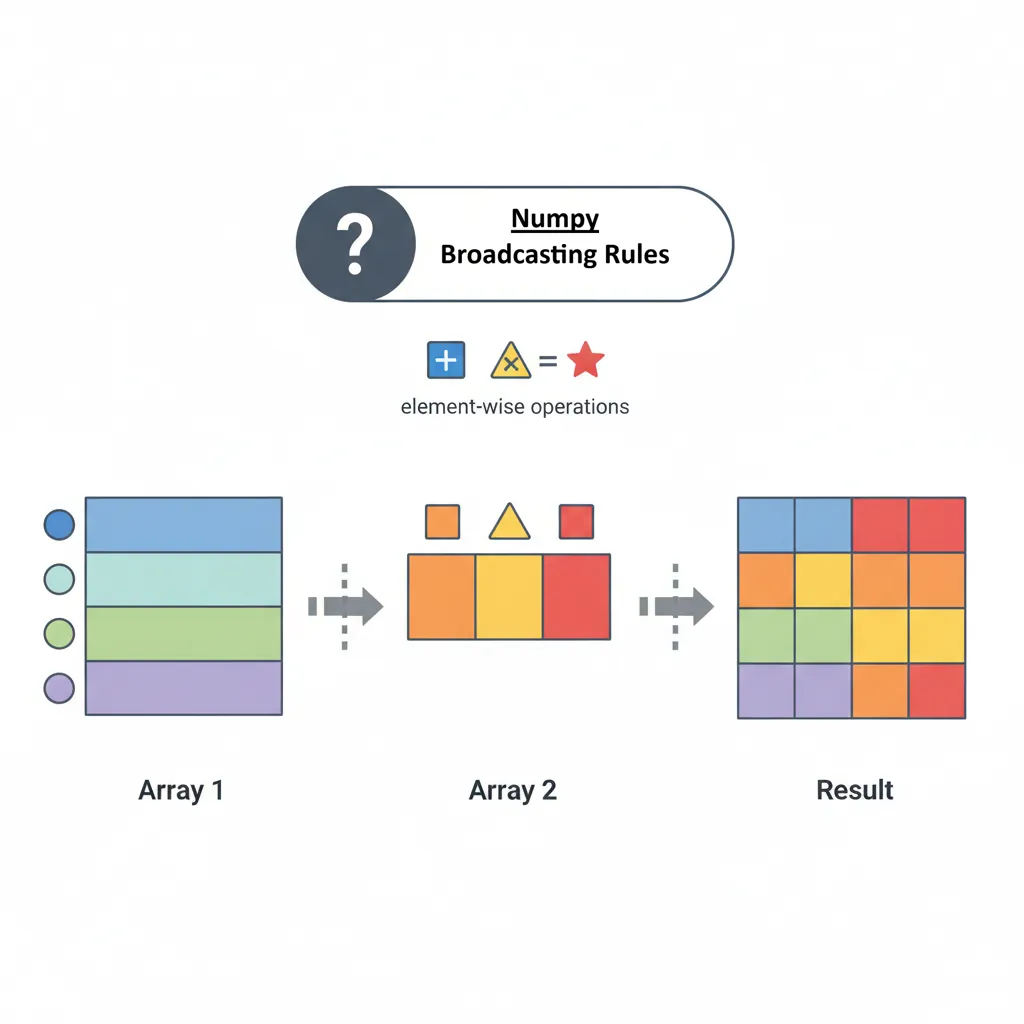
Broadcasting is NumPy's ability to perform operations on arrays of different shapes without explicit loops or copying data. This makes code both faster and more readable.

Broadcasting Rules

NumPy compares shapes element-wise from right to left. Two dimensions are compatible when:

1. They are equal, or
2. One of them is 1

import numpy as np

# Example 1: Scalar broadcasting
arr = np.array([1, 2, 3, 4])
result = arr + 10              # Adds 10 to each element
print(result)                  # [11, 12, 13, 14]

import numpy as np

# Example 2: 1D to 2D broadcasting
matrix = np.array([[1, 2, 3],
                   [4, 5, 6]])
row_vec = np.array([10, 20, 30])

result = matrix + row_vec      # Adds row_vec to each row
print(result)
# [[11, 22, 33],
#  [14, 25, 36]]

Practical Broadcasting Examples

import numpy as np

# Normalize data (zero mean, unit variance)
data = np.array([[1, 2, 3],
                 [4, 5, 6],
                 [7, 8, 9]])

mean = data.mean(axis=0)       # Column means: [4, 5, 6]
std = data.std(axis=0)         # Column stds

normalized = (data - mean) / std
print("Normalized:\n", normalized)

Array Reshaping & Manipulation

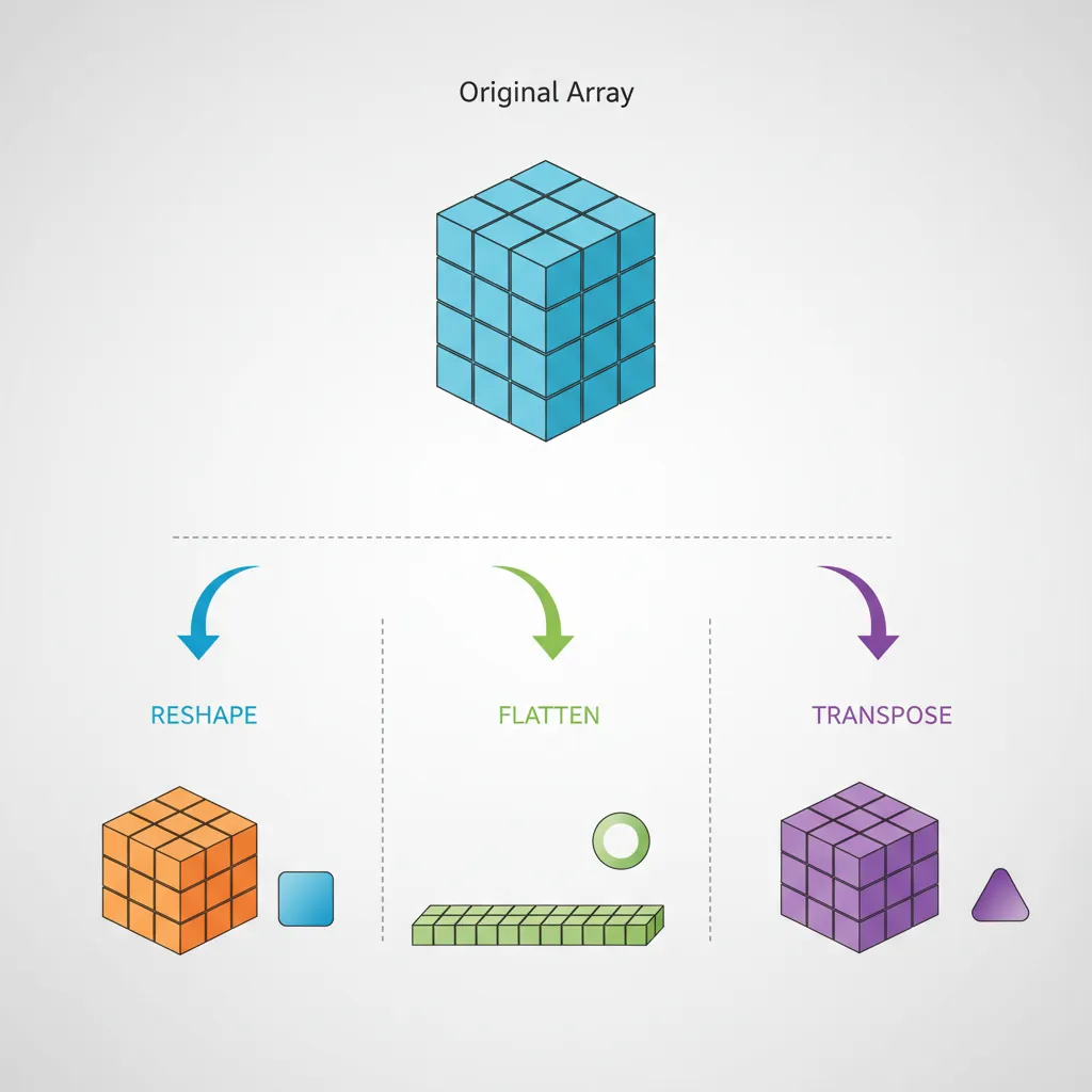
Reshaping arrays is essential for preparing data for different algorithms and transforming between data representations.

Reshaping Arrays

import numpy as np

# Create 1D array
arr = np.arange(12)
print("Original:", arr)          # [0, 1, 2, ..., 11]

# arr.reshape(shape, order='C') - Change array shape without changing data
# Parameters:
#   shape: int or tuple - New dimensions (total elements must match)
#             Use -1 for one dimension to auto-calculate (e.g., (3, -1))
#   order: 'C' or 'F' - Row-major (C) or column-major (Fortran) ordering
# Returns: view if possible, copy if necessary
matrix = arr.reshape(3, 4)       # Reshape to 3x4 (12 elements total)
print("3x4 matrix:\n", matrix)
# [[ 0  1  2  3]
#  [ 4  5  6  7]
#  [ 8  9 10 11]]

import numpy as np

arr = np.arange(12)

# Reshape with -1 (auto-calculate dimension)
# The -1 tells NumPy to figure out this dimension automatically
# Total elements must match: 12 elements = 4 rows × ? columns ? 4 × 3
auto = arr.reshape(4, -1)        # NumPy calculates: (4, 3)
print("Auto reshape shape:", auto.shape)  # (4, 3)
print("Auto reshape:\n", auto)

# Reshape to 3D
# Parameters: (depth, rows, columns) or (blocks, height, width)
cube = arr.reshape(2, 3, 2)      # 2 blocks of 3×2 matrices (2×3×2 = 12 elements)
print("3D shape:", cube.shape)   # (2, 3, 2)
print("2x3x2 cube:\n", cube)

Flattening Arrays

import numpy as np

matrix = np.array([[1, 2, 3], [4, 5, 6]])

# arr.flatten(order='C') - Return 1D copy of array
# Parameters:
#   order: 'C' (row-major, default) or 'F' (column-major)
# Returns: Always creates a NEW copy (safe, but uses more memory)
flat_copy = matrix.flatten()
print("Flatten (copy):", flat_copy)  # [1, 2, 3, 4, 5, 6]
flat_copy[0] = 999                    # Modification doesn't affect original
print("Original unchanged:", matrix[0, 0])  # Still 1

# arr.ravel(order='C') - Return 1D view (if possible)
# Parameters:
#   order: 'C' (row-major, default) or 'F' (column-major)
# Returns: View when possible (faster, less memory), copy when necessary
ravel_view = matrix.ravel()
print("Ravel (view):", ravel_view)   # [1, 2, 3, 4, 5, 6]
ravel_view[0] = 999                   # Modification DOES affect original!
print("Original changed:", matrix[0, 0])  # Now 999

# Key Difference:
# - flatten() always copies (safe but slower)
# - ravel() returns view when possible (faster but modifications propagate)
# Use flatten() when you need independent copy, ravel() for read-only or when you want changes to propagate

Transpose and Swapping Axes

import numpy as np

# arr.T or arr.transpose() - Transpose (swap rows and columns)
# For 2D arrays: .T is shortcut for .transpose()
# Returns: view (not a copy)
A = np.array([[1, 2, 3], [4, 5, 6]])  # Shape (2, 3)
transposed = A.T                       # Shape (3, 2)
print("Original shape:", A.shape)      # (2, 3)
print("Transposed shape:", transposed.shape)  # (3, 2)
print("Transposed:\n", transposed)
# [[1, 4]
#  [2, 5]
#  [3, 6]]

import numpy as np

# arr.transpose(axes=None) - Permute axes for multi-dimensional arrays
# Parameters:
#   axes: tuple of ints - New order of axes (None = reverse all axes)
# For 3D arrays: specify which axis goes where
cube = np.random.rand(2, 3, 4)         # Shape (2, 3, 4)
print("Original shape:", cube.shape)   # (2, 3, 4)

# Swap axes: axis 0 ? 2, axis 1 ? 0, axis 2 ? 1
# Old positions: (0,    1,    2  )
# New positions: (axis2, axis0, axis1) = (2, 0, 1)
swapped = cube.transpose(2, 0, 1)      # (4, 2, 3)
print("Swapped shape:", swapped.shape) # (4, 2, 3)

# Example: Convert (batch, height, width) to (width, batch, height)
# Original: (2, 3, 4) = (batch=2, height=3, width=4)
# Result:   (4, 2, 3) = (width=4, batch=2, height=3)

# np.swapaxes(arr, axis1, axis2) - Swap two specific axes
# Parameters:
#   axis1, axis2: ints - Axes to swap
swapped_simple = np.swapaxes(cube, 0, 2)  # Swap first and last axis
print("Swapaxes (0,2):", swapped_simple.shape)  # (4, 3, 2)

Adding and Removing Dimensions

import numpy as np

# Expand dimensions
arr = np.array([1, 2, 3])
print("Original shape:", arr.shape)  # (3,)

# Add dimension at axis 0
expanded = np.expand_dims(arr, axis=0)
print("Expanded (axis=0):", expanded.shape)   # (1, 3)

# Add dimension at axis 1
expanded = np.expand_dims(arr, axis=1)
print("Expanded (axis=1):", expanded.shape)   # (3, 1)

import numpy as np

# Squeeze: remove single-dimensional entries
arr_with_singles = np.array([[[1, 2, 3]]])
print("Before squeeze:", arr_with_singles.shape)  # (1, 1, 3)
squeezed = np.squeeze(arr_with_singles)
print("After squeeze:", squeezed.shape)          # (3,)

import numpy as np

# Ensure minimum dimensions
x = 5  # scalar
print("atleast_1d:", np.atleast_1d(x).shape)     # (1,)
print("atleast_2d:", np.atleast_2d(x).shape)     # (1, 1)
print("atleast_3d:", np.atleast_3d(x).shape)     # (1, 1, 1)

Tiling and Repeating

import numpy as np

# Tile: repeat entire array
arr = np.array([[1, 2], [3, 4]])
tiled = np.tile(arr, 2)  # Repeat 2 times horizontally
print("Tiled 2x:\n", tiled)
# [[1, 2, 1, 2]
#  [3, 4, 3, 4]]

import numpy as np

arr = np.array([[1, 2], [3, 4]])
tiled = np.tile(arr, (2, 3))  # Repeat 2x vertically, 3x horizontally
print("Tiled (2,3):\n", tiled)

import numpy as np

# Repeat: repeat each element
arr = np.array([1, 2, 3])
repeated = np.repeat(arr, 3)
print("Repeat each 3x:", repeated)  # [1, 1, 1, 2, 2, 2, 3, 3, 3]

import numpy as np

# Repeat along axis
matrix = np.array([[1, 2], [3, 4]])
repeated = np.repeat(matrix, 2, axis=0)
print("Repeat rows:\n", repeated)
# [[1, 2]
#  [1, 2]
#  [3, 4]
#  [3, 4]]

Creating Coordinate Grids

import numpy as np

# Meshgrid: create coordinate matrices for vectorized computations
x = np.array([1, 2, 3])
y = np.array([4, 5])

xx, yy = np.meshgrid(x, y)
print("X grid:\n", xx)
# [[1, 2, 3]
#  [1, 2, 3]]

print("Y grid:\n", yy)
# [[4, 4, 4]
#  [5, 5, 5]]

# Use for function evaluation
z = xx**2 + yy**2
print("f(x,y) = x² + y²:\n", z)

import numpy as np

# mgrid and ogrid for dense/sparse grids
x, y = np.mgrid[0:5, 0:5]  # Dense grid
print("mgrid x shape:", x.shape)  # (5, 5)

x, y = np.ogrid[0:5, 0:5]  # Open (sparse) grid
print("ogrid x shape:", x.shape)  # (5, 1) - memory efficient!

Rearranging Elements

import numpy as np

# Roll: circular shift
arr = np.array([1, 2, 3, 4, 5])
rolled = np.roll(arr, 2)  # Shift right by 2
print("Rolled:", rolled)  # [4, 5, 1, 2, 3]

import numpy as np

# Roll 2D arrays along axis
matrix = np.array([[1, 2, 3], [4, 5, 6]])
rolled = np.roll(matrix, 1, axis=1)  # Shift columns
print("Rolled columns:\n", rolled)
# [[3, 1, 2]
#  [6, 4, 5]]

import numpy as np

# Flip arrays
arr = np.array([1, 2, 3, 4, 5])
flipped = np.flip(arr)
print("Flipped:", flipped)  # [5, 4, 3, 2, 1]

import numpy as np

matrix = np.array([[1, 2], [3, 4]])
print("Flip vertical:\n", np.flipud(matrix))
# [[3, 4]
#  [1, 2]]

print("Flip horizontal:\n", np.fliplr(matrix))
# [[2, 1]
#  [4, 3]]

import numpy as np

# Rotate 90 degrees
matrix = np.array([[1, 2], [3, 4]])
rotated = np.rot90(matrix)
print("Rotated 90°:\n", rotated)
# [[2, 4]
#  [1, 3]]

# Convert 100 28x28 grayscale images to flat vectors
images = np.random.rand(100, 28, 28)
print("Original shape:", images.shape)  # (100, 28, 28)

# Flatten each image: (100, 28, 28) -> (100, 784)
flat_images = images.reshape(100, -1)
print("Flattened shape:", flat_images.shape)  # (100, 784)

# Add channel dimension for CNNs: (100, 28, 28) -> (100, 28, 28, 1)
cnn_images = images.reshape(100, 28, 28, 1)
print("CNN shape:", cnn_images.shape)  # (100, 28, 28, 1)

# Create 2D Gaussian function
x = np.linspace(-3, 3, 100)
y = np.linspace(-3, 3, 100)
xx, yy = np.meshgrid(x, y)

# Evaluate 2D Gaussian: f(x,y) = exp(-(x² + y²)/2)
z = np.exp(-(xx**2 + yy**2) / 2)

print("Grid shape:", xx.shape)  # (100, 100)
print("Z values shape:", z.shape)  # (100, 100)
print("Max value (at origin):", z.max())  # 1.0

# This z array can be directly plotted with matplotlib's contour or imshow

Combining Arrays: Stack & Concatenate

NumPy provides powerful functions to combine multiple arrays in various ways.

Concatenation

import numpy as np

a = np.array([[1, 2], [3, 4]])
b = np.array([[5, 6]])

# Concatenate along rows (axis 0)
vcat = np.concatenate([a, b], axis=0)
print("Vertical concat:\n", vcat)
# [[1, 2]
#  [3, 4]
#  [5, 6]]

# Concatenate along columns (axis 1)
c = np.array([[5], [6]])
hcat = np.concatenate([a, c], axis=1)
print("Horizontal concat:\n", hcat)
# [[1, 2, 5]
#  [3, 4, 6]]

Stacking Functions

import numpy as np

a = np.array([1, 2, 3])
b = np.array([4, 5, 6])

# Vertical stack (row-wise)
vstack = np.vstack([a, b])
print("vstack:\n", vstack)
# [[1, 2, 3]
#  [4, 5, 6]]

# Horizontal stack (column-wise)
hstack = np.hstack([a, b])
print("hstack:", hstack)         # [1, 2, 3, 4, 5, 6]

# Depth stack (3D stacking)
dstack = np.dstack([a, b])
print("dstack shape:", dstack.shape)  # (1, 3, 2)

Column and Row Stack

import numpy as np

a = np.array([1, 2, 3])
b = np.array([4, 5, 6])

# Column stack: 1D arrays -> 2D columns
col_stack = np.column_stack([a, b])
print("Column stack:\n", col_stack)
# [[1, 4]
#  [2, 5]
#  [3, 6]]

# Row stack (alias for vstack)
row_stack = np.row_stack([a, b])
print("Row stack:\n", row_stack)

Splitting Arrays

import numpy as np

# Split array into equal parts
arr = np.array([1, 2, 3, 4, 5, 6])
split_arrays = np.split(arr, 3)  # Split into 3 equal parts
print("Split into 3:", [a for a in split_arrays])
# [array([1, 2]), array([3, 4]), array([5, 6])]

# Split at specific indices
split_arrays = np.split(arr, [2, 4])  # Split at indices 2 and 4
print("Split at indices:", [a for a in split_arrays])
# [array([1, 2]), array([3, 4]), array([5, 6])]

import numpy as np

# Horizontal and vertical splits
matrix = np.array([[1, 2, 3, 4],
                   [5, 6, 7, 8],
                   [9, 10, 11, 12]])

# Split horizontally (column-wise)
h_split = np.hsplit(matrix, 2)
print("Horizontal split:")
for arr in h_split:
    print(arr)
# [[1, 2]    [[3, 4]
#  [5, 6]     [7, 8]
#  [9, 10]]   [11, 12]]

# Split vertically (row-wise)
v_split = np.vsplit(matrix, 3)
print("Vertical split:")
for arr in v_split:
    print(arr)  # [[1,2,3,4]], [[5,6,7,8]], [[9,10,11,12]]

Sorting, Searching & Set Operations

Sorting Arrays

import numpy as np

arr = np.array([3, 1, 4, 1, 5, 9, 2, 6])

# Sort array (returns new sorted array)
sorted_arr = np.sort(arr)
print("Sorted:", sorted_arr)     # [1, 1, 2, 3, 4, 5, 6, 9]

# Argsort (returns indices that would sort the array)
indices = np.argsort(arr)
print("Argsort:", indices)       # [1, 3, 6, 0, 2, 4, 7, 5]
print("Using indices:", arr[indices])  # Same as sorted_arr

import numpy as np

arr = np.array([3, 1, 4, 1, 5, 9, 2, 6])

# Sort in descending order
desc = np.sort(arr)[::-1]
print("Descending:", desc)       # [9, 6, 5, 4, 3, 2, 1, 1]

Sorting 2D Arrays

import numpy as np

matrix = np.array([[3, 1, 4],
                   [1, 5, 9],
                   [2, 6, 5]])

# Sort along axis 0 (columns)
col_sorted = np.sort(matrix, axis=0)
print("Column sorted:\n", col_sorted)

# Sort along axis 1 (rows)
row_sorted = np.sort(matrix, axis=1)
print("Row sorted:\n", row_sorted)

Searching Arrays

import numpy as np

arr = np.array([1, 3, 5, 7, 9, 11])

# Binary search in sorted array
idx = np.searchsorted(arr, 6)
print("Insert position for 6:", idx)  # 3 (between 5 and 7)

# Search for multiple values
indices = np.searchsorted(arr, [4, 8, 10])
print("Insert positions:", indices)  # [2, 4, 5]

# Find where condition is true
greater_than_5 = np.where(arr > 5)
print("Indices > 5:", greater_than_5)  # (array([3, 4, 5]),)

Set Operations

import numpy as np

# Unique values
arr_dup = np.array([1, 2, 2, 3, 3, 3, 4])
unique = np.unique(arr_dup)
print("Unique:", unique)         # [1, 2, 3, 4]

# Unique with counts
unique, counts = np.unique(arr_dup, return_counts=True)
print("Counts:", dict(zip(unique, counts)))  # {1: 1, 2: 2, 3: 3, 4: 1}

import numpy as np

a = np.array([1, 2, 3, 4, 5])
b = np.array([4, 5, 6, 7, 8])

# Set operations
intersection = np.intersect1d(a, b)
print("Intersection:", intersection)  # [4, 5]

union = np.union1d(a, b)
print("Union:", union)           # [1, 2, 3, 4, 5, 6, 7, 8]

difference = np.setdiff1d(a, b)
print("Difference (a-b):", difference)  # [1, 2, 3]

import numpy as np

# Find top 3 scores and their indices
scores = np.array([85, 92, 78, 95, 88, 73, 99, 82])

# Use argpartition for efficient partial sorting
k = 3
top_k_indices = np.argpartition(scores, -k)[-k:]
top_k_scores = scores[top_k_indices]

# Sort the top K in descending order
sorted_idx = top_k_indices[np.argsort(top_k_scores)][::-1]
print("Top 3 scores:", scores[sorted_idx])      # [99, 95, 92]
print("Top 3 indices:", sorted_idx)             # [6, 3, 1]

Statistical Functions

Descriptive Statistics

import numpy as np

data = np.array([85, 92, 78, 95, 88, 73, 99, 82])

# Basic statistics
print("Mean:", data.mean())           # 86.5
print("Median:", np.median(data))     # 86.5
print("Std Dev:", data.std())         # 7.94
print("Variance:", data.var())        # 63.0
print("Min:", data.min())             # 73
print("Max:", data.max())             # 99
print("Range:", data.ptp())           # 26 (peak-to-peak)

Percentiles and Quantiles

import numpy as np

data = np.array([85, 92, 78, 95, 88, 73, 99, 82])

# Percentiles
p25 = np.percentile(data, 25)
p50 = np.percentile(data, 50)  # Same as median
p75 = np.percentile(data, 75)
print(f"25th: {p25}, 50th: {p50}, 75th: {p75}")

# Quantiles (equivalent to percentiles / 100)
q = np.quantile(data, [0.25, 0.5, 0.75])
print("Quantiles:", q)

Correlation and Covariance

import numpy as np

# Two variables
hours_studied = np.array([2, 3, 4, 5, 6, 7, 8])
test_scores = np.array([65, 70, 75, 80, 85, 90, 95])

# Correlation coefficient
correlation = np.corrcoef(hours_studied, test_scores)
print("Correlation matrix:\n", correlation)
print("Correlation:", correlation[0, 1])  # ~1.0 (perfect positive)

# Covariance
covariance = np.cov(hours_studied, test_scores)
print("Covariance matrix:\n", covariance)

Histograms

import numpy as np

# Create histogram data
data = np.random.randn(1000)
counts, bins = np.histogram(data, bins=10)

print("Counts:", counts)
print("Bin edges:", bins)

# Histogram with custom bins
counts, bins = np.histogram(data, bins=[-3, -2, -1, 0, 1, 2, 3])
print("Custom bins counts:", counts)

Saving & Loading Arrays

NumPy provides efficient binary formats for saving and loading arrays, preserving data types and shapes.

Single Array: .npy Format

import numpy as np

# Save single array
data = np.array([[1, 2, 3], [4, 5, 6]])
np.save('my_array.npy', data)

# Load array
loaded = np.load('my_array.npy')
print("Loaded:\n", loaded)
print("Same array:", np.array_equal(data, loaded))  # True

Multiple Arrays: .npz Format

import numpy as np

# Save multiple arrays
x = np.array([1, 2, 3])
y = np.array([4, 5, 6])
z = np.array([[7, 8], [9, 10]])

np.savez('multiple_arrays.npz', x=x, y=y, z=z)

# Load multiple arrays
loaded = np.load('multiple_arrays.npz')
print("Available arrays:", loaded.files)  # ['x', 'y', 'z']
print("X:", loaded['x'])
print("Y:", loaded['y'])
print("Z:", loaded['z'])

Compressed Format: .npz

import numpy as np

# Save compressed (smaller file size)
large_array = np.random.rand(1000, 1000)
np.savez_compressed('compressed.npz', data=large_array)

# Load compressed (transparent decompression)
loaded = np.load('compressed.npz')
print("Shape:", loaded['data'].shape)

Text Files: CSV-like

import numpy as np

# Save to text file
data = np.array([[1, 2, 3], [4, 5, 6]])
np.savetxt('data.txt', data, delimiter=',', fmt='%d')

# Load from text file
loaded = np.loadtxt('data.txt', delimiter=',')
print("Loaded from text:\n", loaded)

import numpy as np
import time

# Create large array
large = np.random.rand(10000, 100)

# Binary save (.npy) - FAST
start = time.time()
np.save('binary.npy', large)
binary_time = time.time() - start

# Text save (.txt) - SLOW
start = time.time()
np.savetxt('text.txt', large)
text_time = time.time() - start

print(f"Binary save: {binary_time:.3f}s")
print(f"Text save: {text_time:.3f}s")
print(f"Binary is {text_time/binary_time:.1f}x faster")

Linear Algebra Operations

NumPy's linalg module provides comprehensive linear algebra functionality essential for machine learning and scientific computing.

Matrix Operations

import numpy as np

A = np.array([[1, 2], [3, 4]])
B = np.array([[5, 6], [7, 8]])

# Matrix multiplication
C = A @ B                      # Python 3.5+ syntax
# or: C = np.dot(A, B)
print("A @ B:\n", C)

# Transpose
print("Transpose:\n", A.T)

# Determinant
det = np.linalg.det(A)
print("Determinant:", det)     # -2.0

# Inverse (if exists)
A_inv = np.linalg.inv(A)
print("Inverse:\n", A_inv)

Eigenvalues and Eigenvectors

import numpy as np

matrix = np.array([[4, -2],
                   [1,  1]])

eigenvalues, eigenvectors = np.linalg.eig(matrix)
print("Eigenvalues:", eigenvalues)
print("Eigenvectors:\n", eigenvectors)

import numpy as np

# Generate synthetic data
X = np.array([[1, 1], [1, 2], [1, 3]])  # Features with bias term
y = np.array([2, 4, 6])                  # Target values

# Normal equation: theta = (X^T X)^(-1) X^T y
theta = np.linalg.inv(X.T @ X) @ X.T @ y
print("Coefficients:", theta)            # [0, 2] (intercept=0, slope=2)

Random Number Generation

NumPy's random module is crucial for simulations, data generation, and machine learning initialization.

Basic Random Generation

import numpy as np

# np.random.seed(seed) - Set random number generator seed for reproducibility
# Parameters:
#   seed: int - Seed value (same seed = same random sequence)
np.random.seed(42)

# np.random.rand(d0, d1, ..., dn) - Random floats from uniform [0, 1)
# Parameters:
#   d0, d1, ..., dn: ints - Dimensions of output array
#   Returns: floats in range [0.0, 1.0)
uniform = np.random.rand(3, 3)         # 3x3 array of random floats
print("Uniform [0,1):\n", uniform)

# np.random.randint(low, high=None, size=None, dtype=int) - Random integers
# Parameters:
#   low: int - Lowest integer (inclusive), or if high=None, range is [0, low)
#   high: int - Highest integer (exclusive)
#   size: int or tuple - Shape of output array
#   dtype: data type - Integer type (default: int)
integers = np.random.randint(0, 10, size=(2, 3))  # Random ints from 0 to 9
print("Random integers:\n", integers)

# np.random.randn(d0, d1, ..., dn) - Random floats from standard normal (mean=0, std=1)
# Parameters:
#   d0, d1, ..., dn: ints - Dimensions of output array
#   Returns: samples from normal distribution N(0, 1)
normal = np.random.randn(1000)         # 1000 samples from standard normal
print("Normal mean:", normal.mean())    # ~0
print("Normal std:", normal.std())      # ~1

Statistical Distributions

import numpy as np

# np.random.exponential(scale=1.0, size=None) - Exponential distribution
# Parameters:
#   scale: float - Scale parameter (1/lambda, mean of distribution)
#   size: int or tuple - Output shape
exponential = np.random.exponential(scale=2.0, size=1000)
print(f"Exponential mean: {exponential.mean():.2f}")  # Should be ~2.0

# np.random.poisson(lam=1.0, size=None) - Poisson distribution (count data)
# Parameters:
#   lam: float - Expected number of events (lambda parameter)
#   size: int or tuple - Output shape
poisson = np.random.poisson(lam=3, size=1000)
print(f"Poisson mean: {poisson.mean():.2f}")  # Should be ~3.0

# np.random.binomial(n, p, size=None) - Binomial distribution (coin flips)
# Parameters:
#   n: int - Number of trials
#   p: float - Probability of success (0 to 1)
#   size: int or tuple - Output shape
binomial = np.random.binomial(n=10, p=0.5, size=1000)  # 10 coin flips, 1000 times
print(f"Binomial mean: {binomial.mean():.2f}")  # Should be ~5.0 (n*p)

# np.random.shuffle(x) - Shuffle array in-place (modifies original)
# Parameters:
#   x: array - Array to shuffle (modified directly)
deck = np.arange(52)                   # Create deck [0, 1, 2, ..., 51]
np.random.shuffle(deck)                # Shuffle in-place
print(f"First 5 cards after shuffle: {deck[:5]}")

# np.random.choice(a, size=None, replace=True, p=None) - Random sample from array
# Parameters:
#   a: array or int - If int, sample from range(a); if array, sample from array
#   size: int or tuple - Output shape
#   replace: bool - Sample with replacement (True) or without (False)
#   p: array - Probabilities for each element (must sum to 1)
hand = np.random.choice(deck, size=5, replace=False)  # Draw 5 unique cards
print(f"Hand: {hand}")

Performance Optimization

Views vs Copies

Understanding when NumPy creates views (references) versus copies is critical for performance:

import numpy as np

original = np.array([1, 2, 3, 4, 5])

# Slicing creates a VIEW (shares memory)
view = original[1:4]
view[0] = 999
print("Original changed:", original)  # [1, 999, 3, 4, 5]

# Fancy indexing creates a COPY
copy = original[[0, 2, 4]]
copy[0] = 777
print("Original unchanged:", original)  # [1, 999, 3, 4, 5]

Memory Layout: C vs Fortran Order

import numpy as np

# C-contiguous (row-major, default)
c_array = np.array([[1, 2], [3, 4]], order='C')

# Fortran-contiguous (column-major)
f_array = np.array([[1, 2], [3, 4]], order='F')

# Check with flags
print("C-contiguous:", c_array.flags['C_CONTIGUOUS'])
print("F-contiguous:", f_array.flags['F_CONTIGUOUS'])

import numpy as np
import time

size = 1_000_000
a = np.random.rand(size)
b = np.random.rand(size)

# Python loop approach
start = time.time()
result = []
for i in range(size):
    result.append(a[i] + b[i])
python_time = time.time() - start

# NumPy vectorized approach
start = time.time()
result_np = a + b
numpy_time = time.time() - start

print(f"Python loop: {python_time:.4f}s")
print(f"NumPy vectorized: {numpy_time:.4f}s")
print(f"Speedup: {python_time/numpy_time:.1f}x")

Practical Applications

Image Processing

Images are just 3D arrays (height × width × channels):

import numpy as np

# Simulate a 100x100 RGB image
image = np.random.randint(0, 256, size=(100, 100, 3), dtype=np.uint8)

# Convert to grayscale (weighted average)
gray = np.dot(image[...,:3], [0.299, 0.587, 0.114])

# Flip horizontally
flipped = image[:, ::-1, :]

# Crop center
h, w = image.shape[:2]
cropped = image[h//4:3*h//4, w//4:3*w//4, :]

Statistical Analysis

import numpy as np

# Generate sample data
data = np.random.normal(loc=100, scale=15, size=1000)

# Compute statistics
mean = data.mean()
median = np.median(data)
std = data.std()
percentiles = np.percentile(data, [25, 50, 75])

print(f"Mean: {mean:.2f}")
print(f"Median: {median:.2f}")
print(f"Std Dev: {std:.2f}")
print(f"IQR: {percentiles[2] - percentiles[0]:.2f}")

Time Series Analysis

import numpy as np

# Moving average
def moving_average(data, window):
    return np.convolve(data, np.ones(window)/window, mode='valid')

prices = np.random.randn(100).cumsum() + 100
ma_5 = moving_average(prices, 5)
ma_20 = moving_average(prices, 20)

Next Steps in the Series

Congratulations! You now understand NumPy's core concepts and capabilities. You've mastered:

• ? Array creation and manipulation
• ? Vectorized operations and broadcasting
• ? Indexing, slicing, and boolean masking
• ? Linear algebra operations
• ? Performance optimization techniques

NumPy is the foundation, but Pandas is where data science really comes alive. See you in the next article!

NumPy API Cheat Sheet

Quick reference for the most commonly used NumPy operations covered in this article.