We use cookies to enhance your browsing experience, serve personalized content, and analyze our traffic.
By clicking "Accept All", you consent to our use of cookies. See our
Privacy Policy
for more information.
Python Data Science Series Part 2: Pandas for Data Analysis
December 27, 2025Wasil Zafar22 min read
Master Pandas, Python's primary tool for data manipulation and analysis. Learn DataFrames, Series, data cleaning, transformation, groupby operations, and everything needed for real-world data work.
Prerequisites: Before running the code examples in this tutorial, make sure you have Python and Jupyter notebooks properly set up. If you haven't configured your development environment yet, check out our complete setup guide for VS Code, PyCharm, Jupyter, and Colab.
If NumPy is the foundation of Python's data science stack, Pandas is where data analysis truly begins. Built on top of NumPy, Pandas provides high-level data structures and tools specifically designed for working with real-world, tabular data—the kind you find in spreadsheets, databases, and CSV files.
Why Pandas Matters: Pandas is to data science what SQL is to databases—the essential tool for data manipulation. It's the first library you reach for when loading, cleaning, transforming, and analyzing data before machine learning or visualization.
DataFrame: 2D table with labeled rows and columns (like Excel, but programmable)
Series: 1D labeled array (a single column or row)
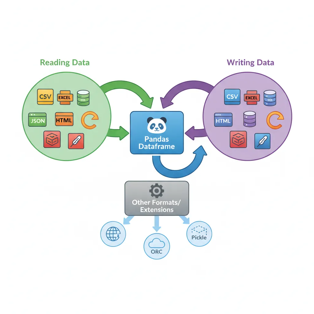
I/O tools: Read/write CSV, Excel, JSON, SQL, Parquet, and more
Data cleaning: Handle missing values, duplicates, and transformations
GroupBy: Split-apply-combine operations for aggregation
Merge/Join: Combine datasets like SQL joins
Time series: Specialized support for datetime data
Installation and Setup
# Install Pandas
pip install pandas

# Import convention
import pandas as pd
import numpy as np

print(f"pandas version: {pd.__version__}")
Series: 1D Labeled Arrays
A Series is a one-dimensional labeled array—like a column in a spreadsheet or a single feature in a dataset. It combines NumPy's array performance with labeled indices.
Figure 1: Anatomy of a Pandas Series — labeled index paired with a NumPy array of values
import pandas as pd
import numpy as np

# Creating Series from list
s = pd.Series([10, 20, 30, 40], index=['a', 'b', 'c', 'd'], name='scores')
print(s)
# Output:
# a    10
# b    20
# c    30
# d    40
# Name: scores, dtype: int64

# Access by label and position
print("By label 'b':", s['b'])     # 20
print("By position 2:", s.iloc[2]) # 30

# Vectorized operations
print("Add 5:", s + 5)
print("Multiply by 2:", s * 2)
Index Alignment
Pandas automatically aligns data by index labels—a powerful feature:
import pandas as pd

s1 = pd.Series([1, 2, 3], index=['a', 'b', 'c'])
s2 = pd.Series([10, 20, 30], index=['b', 'c', 'd'])

# Alignment by index (missing indices become NaN)
result = s1 + s2
print(result)
# a     NaN
# b    12.0
# c    23.0
# d     NaN
Critical Concept: Index alignment happens automatically. Operations match by labels, not positions. This prevents silent bugs when working with mismatched data but can introduce NaN values.
DataFrame: 2D Tabular Data
The DataFrame is Pandas' primary data structure—a 2D table with labeled rows and columns. Think of it as a spreadsheet or SQL table in Python.
import pandas as pd

# Create DataFrame from dictionary
df = pd.DataFrame({
    'name': ['Alice', 'Bob', 'Charlie', 'Diana'],
    'age': [25, 30, 35, 28],
    'city': ['NY', 'LA', 'NY', 'SF'],
    'score': [88, 92, 85, 90]
})

print(df)
#       name  age city  score
# 0    Alice   25   NY     88
# 1      Bob   30   LA     92
# 2  Charlie   35   NY     85
# 3    Diana   28   SF     90

# Data inspection
print(df.head(2))        # First 2 rows
print(df.info())         # Structure and types
print(df.describe())     # Statistical summary
print(df.shape)          # (4, 4) - rows × columns
Column Operations
import pandas as pd

df = pd.DataFrame({
    'name': ['Alice', 'Bob', 'Charlie', 'Diana'],
    'age': [25, 30, 35, 28],
    'city': ['NY', 'LA', 'NY', 'SF'],
    'score': [88, 92, 85, 90]
})

# Select single column (returns Series)
ages = df['age']
print(type(ages))  #

# Select multiple columns (returns DataFrame)
subset = df[['name', 'score']]

# Add new column
df['is_ny'] = df['city'] == 'NY'
print(df)
#       name  age city  score  is_ny
# 0    Alice   25   NY     88   True
# 1      Bob   30   LA     92  False
# 2  Charlie   35   NY     85   True
# 3    Diana   28   SF     90  False
DataFrame Anatomy
Understanding DataFrame Structure
Index: Row labels (default: 0, 1, 2, ...)
Columns: Column labels (from keys or specified)
Values: Underlying NumPy array (access with .values)
dtypes: Data type per column (int64, float64, object)
When working with NumPy arrays or numerical DataFrames, you can use boolean indexing on multiple dimensions—a powerful technique for filtering machine learning datasets by class or condition.
import pandas as pd
import numpy as np

# Create a dataset with features (X) and labels (y)
X = np.array([[1.2, 2.3, 3.1],
              [4.5, 5.6, 6.2],
              [7.8, 8.9, 9.3],
              [2.1, 3.4, 4.5],
              [5.6, 6.7, 7.8]])

y = np.array([0, 1, 1, 0, 1])  # Binary labels (class 0 or 1)

print("Full dataset:")
print("X shape:", X.shape)  # (5, 3)
print("y shape:", y.shape)  # (5,)
print("X:\n", X)
print("y:", y)
Filtering Rows by Class Label
The syntax X[y==0] creates a boolean mask and applies it to select rows:
Chained assignment can produce a copy instead of a view, causing silent failures. Always use .loc for assignments.
Practice Exercises
Selection & Filtering Exercises
Exercise 1 (Beginner): Create a DataFrame with columns name, age, city, salary. Select all rows where age > 30. Select only name and salary columns for these rows.
Exercise 2 (Beginner): Create a DataFrame. Add a new column 'bonus' that is 10% of salary. Modify existing columns using .loc[]. Check the difference between copy() and view.
Exercise 3 (Intermediate): Create a DataFrame. Filter rows where (city == 'NY') AND (salary > 50000). Try boolean operators (&, |, ~). Explain what goes wrong with 'and' operator.
Exercise 4 (Intermediate): Create a DataFrame with various data types (int, float, string, bool). Use iloc for position-based selection. Extract specific rows and columns by integer position.
Challenge (Advanced): Create a DataFrame and use query() method for complex conditions. Compare performance and readability with .loc[] approach on large data.
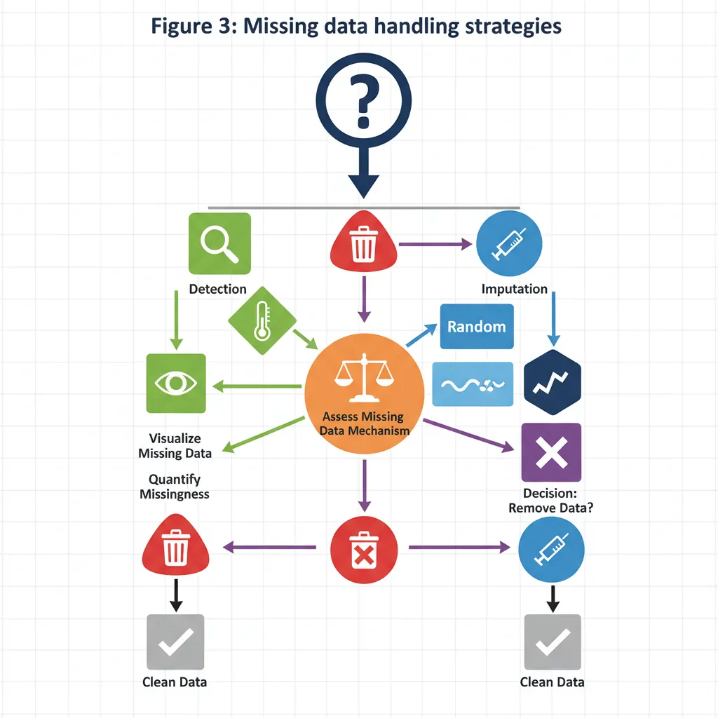
Handling Missing Data
Real-world data always has missing values. Pandas provides comprehensive tools to detect, remove, and fill them.
Figure 3: Missing data handling strategies — detection, removal, and imputation decision workflow
import pandas as pd
import numpy as np

df_na = pd.DataFrame({
    'A': [1, np.nan, 3, np.nan],
    'B': ['x', 'y', None, 'z'],
    'C': [10.0, 11.5, np.nan, 9.8]
})

# Detect missing values
print(df_na.isnull())
#        A      B      C
# 0  False  False  False
# 1   True  False  False
# 2  False   True   True
# 3   True  False  False

print(df_na.isnull().sum())  # Count per column
# A    2
# B    1
# C    1
Removing Missing Data
import pandas as pd
import numpy as np

df_na = pd.DataFrame({
    'A': [1, np.nan, 3, np.nan],
    'B': ['x', 'y', None, 'z'],
    'C': [10.0, 11.5, np.nan, 9.8]
})

# Drop rows with ANY missing value
df_clean = df_na.dropna()

# Drop rows where ALL values are missing
df_clean = df_na.dropna(how='all')

# Drop columns with missing values
df_clean = df_na.dropna(axis=1)

# Drop rows missing values in specific columns
df_clean = df_na.dropna(subset=['A', 'C'])
Filling Missing Data
import pandas as pd
import numpy as np

df_na = pd.DataFrame({
    'A': [1, np.nan, 3, np.nan],
    'B': ['x', 'y', None, 'z'],
    'C': [10.0, 11.5, np.nan, 9.8]
})

# Fill with specific value
df_filled = df_na.fillna(0)

# Fill with column means
df_filled = df_na.fillna(df_na.mean())

# Fill with different values per column
df_filled = df_na.fillna({
    'A': df_na['A'].mean(),
    'B': 'missing',
    'C': df_na['C'].median()
})

# Forward fill (propagate last valid value)
df_filled = df_na.fillna(method='ffill')

# Backward fill
df_filled = df_na.fillna(method='bfill')
Best Practice: Never blindly drop or fill missing data. Understand why data is missing (random, systematic, measurement error) before choosing a strategy. Document your decisions.
Operations & Computations
Apply, Map, and Applymap
import pandas as pd

df = pd.DataFrame({
    'name': ['Alice', 'Bob', 'Charlie', 'Diana'],
    'age': [25, 30, 35, 28],
    'city': ['NY', 'LA', 'NY', 'SF'],
    'score': [88, 92, 85, 90]
})

# apply() on columns
df['age_squared'] = df['age'].apply(lambda x: x ** 2)

# apply() on rows (axis=1)
df['total'] = df.apply(lambda row: row['age'] + row['score'], axis=1)

# map() for Series element-wise transformation
city_map = {'NY': 'New York', 'LA': 'Los Angeles', 'SF': 'San Francisco'}
df['city_full'] = df['city'].map(city_map)

# applymap() for entire DataFrame (deprecated, use .map() instead)
df_str = pd.DataFrame({'x': ['a', 'bb'], 'y': ['ccc', 'd']})
lengths = df_str.map(len)  # Apply len to every cell
String Operations
The .str accessor provides vectorized string methods:
Exercise 1 (Beginner): Create a DataFrame with a string column. Use .str.lower(), .str.upper(), .str.title() to transform the text. Print results.
Exercise 2 (Beginner): Create a DataFrame with email addresses. Use .str.contains() to find emails from a specific domain. Use .str.extract() to extract the domain name.
Exercise 3 (Intermediate): Create a DataFrame with names like ' john doe ', 'jane SMITH'. Clean using .str.strip() and .str.title(). Split into first and last names using .str.split().
Exercise 4 (Intermediate): Create a DataFrame with text containing special characters. Use .str.replace() to replace patterns. Use .str.startswith() and .str.endswith() for filtering.
Challenge (Advanced): Create a DataFrame with mixed-case email addresses. Extract domain and user parts separately using .str.extract() with regex groups. Validate email format using .str.match().
Pivot tables reshape data from long to wide format, aggregating as needed—like Excel pivot tables.
import pandas as pd

df = pd.DataFrame({
    'name': ['Alice', 'Bob', 'Charlie', 'Diana'],
    'age': [25, 30, 35, 28],
    'city': ['NY', 'LA', 'NY', 'SF'],
    'score': [88, 92, 85, 90]
})
df['is_ny'] = df['city'] == 'NY'

# Pivot table: reshape and aggregate
pivot = pd.pivot_table(
    df,
    values='score',
    index='city',
    columns='age',
    aggfunc='mean',
    fill_value=0
)
print(pivot)
#       age  25  28  30  35
# city
# LA          0   0  92   0
# NY         88   0   0  85
# SF          0  90   0   0

# Crosstab: frequency table
ct = pd.crosstab(df['city'], df['is_ny'])
print(ct)
# is_ny  False  True
# city
# LA         1     0
# NY         0     2
# SF         1     0
Practice Exercises
GroupBy & Aggregations Exercises
Exercise 1 (Beginner): Create a sales DataFrame with columns: product, region, amount. Group by region and calculate total amount per region. Then group by product.
Exercise 2 (Beginner): Create a DataFrame with numeric columns. Group by a category column and apply multiple aggregations (mean, sum, min, max) simultaneously.
Exercise 3 (Intermediate): Create sales data with date and region. Group by region and month, then calculate total revenue. Use unstack() to create a pivot-like view.
Exercise 4 (Intermediate): Write a custom aggregation function (e.g., coefficient of variation) and apply it to grouped data. Compare with built-in agg functions.
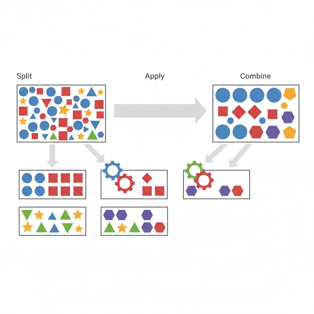
Challenge (Advanced): Create complex grouped data. Use transform() to add group means as a new column. Use apply() for custom group-wise transformations. Explain difference from agg().
Merge, Join & Concatenate
Combining datasets is crucial for data analysis. Pandas provides SQL-like joins and concatenation.
Figure 5: Pandas merge join types — inner, left, right, and outer joins visualized as set operations
Merge (SQL-style joins)
import pandas as pd

left = pd.DataFrame({'id': [1, 2, 3], 'city': ['NY', 'LA', 'SF']})
right = pd.DataFrame({'id': [1, 2, 4], 'score': [88, 92, 77]})

# Inner join (intersection)
inner = left.merge(right, on='id', how='inner')
print(inner)
#    id city  score
# 0   1   NY     88
# 1   2   LA     92

# Left join (all from left, matching from right)
left_join = left.merge(right, on='id', how='left')
print(left_join)
#    id city  score
# 0   1   NY   88.0
# 1   2   LA   92.0
# 2   3   SF    NaN

# Outer join (all from both)
outer = left.merge(right, on='id', how='outer')
print(outer)
Join (index-based)
import pandas as pd

left = pd.DataFrame({'id': [1, 2, 3], 'city': ['NY', 'LA', 'SF']})
right = pd.DataFrame({'id': [1, 2, 4], 'score': [88, 92, 77]})

l = left.set_index('id')
r = right.set_index('id')

# Join on index
joined = l.join(r, how='left')
print(joined)
✅ Use categorical dtype for repeated labels to save memory
Common Pitfalls
Avoid These Mistakes
Chained assignment: Use .loc instead of df[cond][col] = val
Ignoring dtypes: Check and convert types explicitly
Not setting index: Use meaningful indices for time series and joins
Copying unnecessarily: Many operations return views—use .copy() when needed
Mixing label/position indexing: Stick to loc or iloc, don't mix
What's Next
You've mastered Pandas—data loading, cleaning, transformation, grouping, and merging. You're now ready to visualize your insights!
Practice Exercises
Merge & Join Exercises
Exercise 1 (Beginner): Create two DataFrames with overlapping IDs. Perform inner, outer, left, and right joins. Compare row counts and identify missing data.
Exercise 2 (Beginner): Create customer and order DataFrames. Merge on customer_id. Then group by customer to calculate total purchases.
Exercise 3 (Intermediate): Create multiple DataFrames. Concatenate them vertically (vstack) and horizontally (hstack). Use ignore_index=True. Explain when to use which.
Exercise 4 (Intermediate): Create DataFrames with non-matching keys. Try merging on key using how='left'. Handle NaN values from unmatched rows using fillna().
Challenge (Advanced): Create 3+ DataFrames with different keys. Chain multiple merges or use reduce() to combine all. Verify final row count matches expected result.
Pandas API Cheat Sheet
Quick reference for essential Pandas operations for data manipulation and analysis.
DataFrame Creation
pd.DataFrame(dict)
From dictionary
pd.read_csv('file.csv')
From CSV file
pd.read_excel('file.xlsx')
From Excel
pd.read_json('file.json')
From JSON
pd.read_sql(query, conn)
From SQL query
pd.Series([1,2,3])
Create Series
Data Inspection
df.head(n)
First n rows
df.tail(n)
Last n rows
df.info()
Column types & nulls
df.describe()
Statistical summary
df.shape
(rows, columns)
df.dtypes
Column data types
Selection & Filtering
df['col']
Select column
df[['a','b']]
Select columns
df.loc['idx']
By label
df.iloc[0]
By position
df[df['age'] > 25]
Boolean filter
df.query('age > 25')
Query syntax
df.isin(['NY','LA'])
Membership test
Missing Data
df.isnull()
Detect NaN values
df.isnull().sum()
Count nulls per col
df.dropna()
Drop rows with NaN
df.fillna(value)
Fill with value
df.fillna(method='ffill')
Forward fill
df.fillna(df.mean())
Fill with mean
GroupBy & Aggregation
df.groupby('col')
Group by column
.mean()
Group mean
.sum()
Group sum
.count()
Group count
.agg(['min','max'])
Multiple aggs
.transform(fn)
Broadcast result
pd.pivot_table()
Pivot & aggregate
Merging & Joining
pd.merge(df1, df2)
Merge (inner)
how='left'
Left join
how='right'
Right join
how='outer'
Outer join
on='key'
Merge on column
df1.join(df2)
Join on index
pd.concat([df1,df2])
Stack DataFrames
Transformation
df['new'] = df['a'] + df['b']
Add column
df.apply(fn)
Apply function
df['col'].map(dict)
Map values
df.sort_values('col')
Sort by column
df.rename(columns={})
Rename columns
df.drop(['col'], axis=1)
Drop column
df.reset_index()
Reset index
String Operations
df['col'].str.lower()
To lowercase
.str.upper()
To uppercase
.str.strip()
Remove whitespace
.str.contains('word')
Contains pattern
.str.startswith('A')
Starts with
.str.split(',')
Split string
.str.replace('old','new')
Replace text
Pro Tips:
loc vs iloc:loc uses labels, iloc uses positions (integers)
Chaining: Avoid chained assignment; use .loc[] for safe updates
Method chaining: Chain methods for cleaner code: df.dropna().groupby('col').mean()
Performance: Use vectorized operations instead of .apply() when possible
Related Articles in This Series
Part 1: NumPy Foundations for Data Science
Master NumPy arrays, vectorization, broadcasting, and linear algebra operations—the foundation of Python data science.
Part 3: Data Visualization with Matplotlib & Seaborn
Create compelling visualizations with Python's most powerful plotting libraries. Learn line plots, bar charts, scatter plots, and statistical graphics.