DSA Part 12: Graph Traversal & Representations

                Mastery target: Level A recognition, progressing toward Level B implementation. You should be able to choose a graph representation from its access pattern, and trace BFS and DFS by hand before writing either from memory.
            

1. Why Graphs, Why Now

Parts 9 through 11 covered trees and heaps: structures with a single root, a fixed shape, and a clear notion of "up" and "down". Graphs drop those constraints. A graph is any collection of nodes and the connections between them, with no required root, no required hierarchy, and no limit on how many neighbors a node can have. A tree is simply a graph with no cycles and exactly one path between any two nodes - graphs are the more general model underneath social networks, road maps, dependency chains, and program call graphs.

This lesson is Part 12 of the Interview Foundations core series - previously an overloaded page that joined graphs, dynamic programming, greedy algorithms, and backtracking into a single lesson. That page is being split into six focused units so each algorithm family gets its own mental model and worked trace. This is the first: graph representations and the two traversal algorithms, BFS and DFS, that almost every other graph algorithm builds on.

2. Prerequisites

Two earlier lessons matter directly here. Read them first if either feels shaky:

Part 2: Recursion Complete Guide - recursive DFS is just a call-stack trace. If tracing recursive calls and base cases is not yet automatic, review it before the DFS section below.
Part 3: Arrays & Array ADT - the Number of Islands problem treats a 2D array as an implicit graph, where each cell is a node and its up/down/left/right neighbors are edges. Comfort with 2D array indexing and bounds checking is assumed.

3. Graph Fundamentals

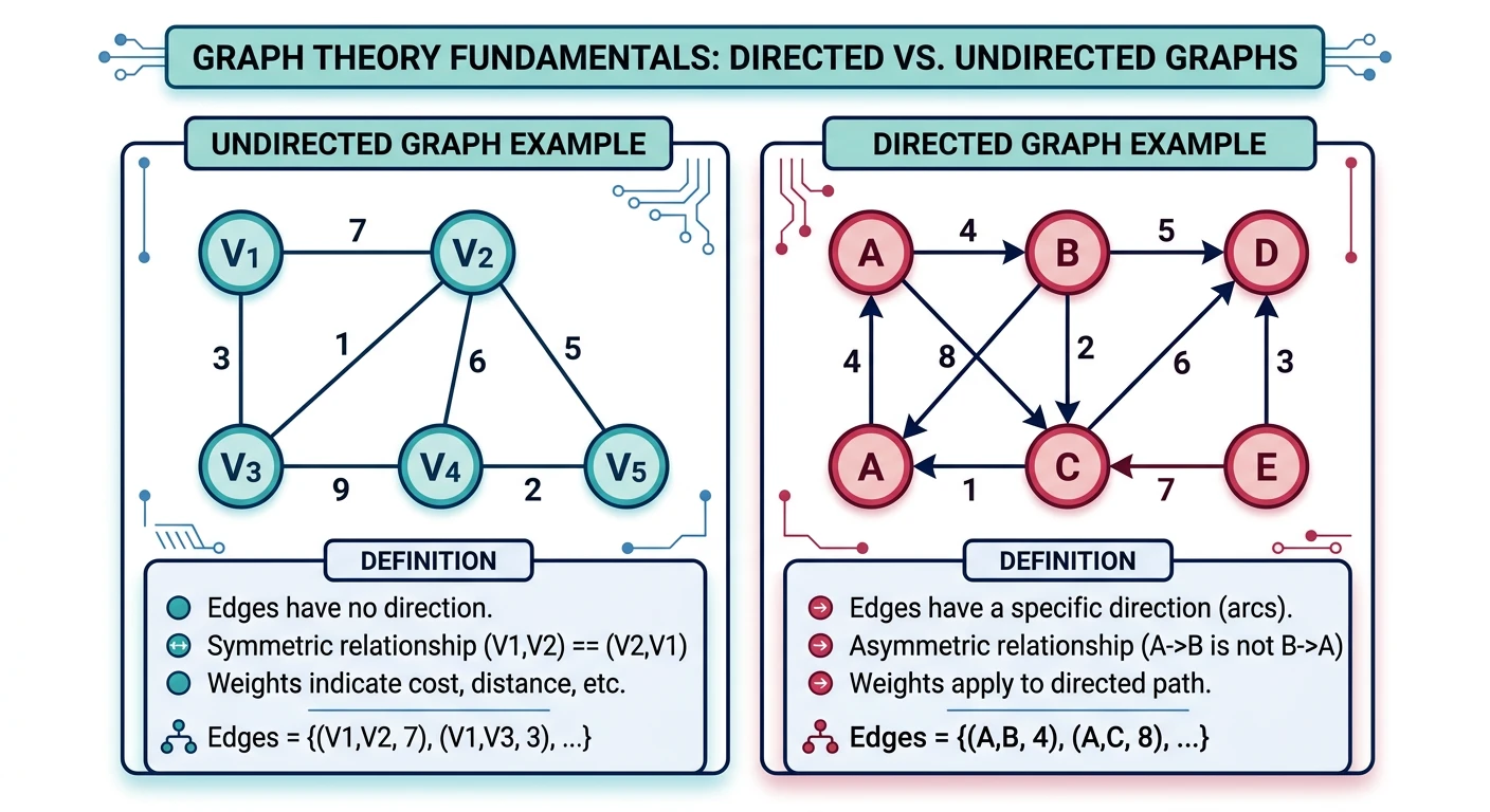
A Graph is a collection of nodes (vertices) and edges connecting them. Graphs model relationships and networks, appearing frequently in interview problems.

Directed and undirected graph examples with vertices, edges, and weights labeled — Graph types: undirected graph with bidirectional edges, directed graph with one-way edges, and weighted graph with edge costs

                            Graph Terminology
                            Directed: Edges have direction (A→B)
Undirected: Edges go both ways (A—B)
Weighted: Edges have costs/weights
Cycle: Path that starts and ends at same node
Connected: Path exists between all vertex pairs

                        

Graph Representations

Choosing the right representation determines the efficiency of every graph algorithm. The Adjacency List maps each vertex to a list of its neighbors — space-efficient for sparse graphs ($O(V + E)$ space) and fast neighbor iteration. It's the default choice for most interview and production scenarios.

from collections import defaultdict

# 1. Adjacency List (most common for sparse graphs)
class GraphAdjList:
    """
    Adjacency List representation
    Space: O(V + E)
    Best for: sparse graphs, most interview problems
    """
    def __init__(self, directed=False):
        self.graph = defaultdict(list)
        self.directed = directed

    def add_edge(self, u, v, weight=1):
        self.graph[u].append((v, weight))
        if not self.directed:
            self.graph[v].append((u, weight))

    def get_neighbors(self, u):
        return self.graph[u]

    def __str__(self):
        return str(dict(self.graph))

# Example
g = GraphAdjList(directed=False)
g.add_edge(0, 1)
g.add_edge(0, 2)
g.add_edge(1, 2)
g.add_edge(2, 3)

print("Adjacency List:", g)
print("Neighbors of 0:", g.get_neighbors(0))

// Graph Adjacency List - O(V + E) space
#include <vector>
#include <unordered_map>
#include <iostream>

class GraphAdjList {
private:
    std::unordered_map<int, std::vector<std::pair<int, int>>> graph;
    bool directed;

public:
    GraphAdjList(bool isDirected = false) : directed(isDirected) {}

    void addEdge(int u, int v, int weight = 1) {
        graph[u].push_back({v, weight});
        if (!directed) {
            graph[v].push_back({u, weight});
        }
    }

    std::vector<std::pair<int, int>>& getNeighbors(int u) {
        return graph[u];
    }

    void display() {
        for (auto& [node, neighbors] : graph) {
            std::cout << node << ": ";
            for (auto& [v, w] : neighbors)
                std::cout << "(" << v << "," << w << ") ";
            std::cout << std::endl;
        }
    }
};

// Graph Adjacency List - O(V + E) space
import java.util.*;

class GraphAdjList {
    private Map<Integer, List<int[]>> graph;
    private boolean directed;

    public GraphAdjList(boolean directed) {
        this.graph = new HashMap<>();
        this.directed = directed;
    }

    public void addEdge(int u, int v, int weight) {
        graph.computeIfAbsent(u, k -> new ArrayList<>()).add(new int[]{v, weight});
        if (!directed) {
            graph.computeIfAbsent(v, k -> new ArrayList<>()).add(new int[]{u, weight});
        }
    }

    public void addEdge(int u, int v) { addEdge(u, v, 1); }

    public List<int[]> getNeighbors(int u) {
        return graph.getOrDefault(u, new ArrayList<>());
    }
}

The Adjacency Matrix stores a $V \times V$ boolean/weight matrix where entry $[i][j]$ indicates an edge from $i$ to $j$. It enables $O(1)$ edge existence checks and is ideal for dense graphs (where $E \approx V^2$) or algorithms like Floyd-Warshall that iterate over all pairs. The tradeoff is $O(V^2)$ space regardless of actual edge count.

import numpy as np

# 2. Adjacency Matrix (good for dense graphs)
class GraphAdjMatrix:
    """
    Adjacency Matrix representation
    Space: O(V²)
    Best for: dense graphs, quick edge lookups
    """
    def __init__(self, num_vertices):
        self.V = num_vertices
        self.matrix = [[0] * num_vertices for _ in range(num_vertices)]

    def add_edge(self, u, v, weight=1):
        self.matrix[u][v] = weight
        self.matrix[v][u] = weight  # For undirected

    def has_edge(self, u, v):
        return self.matrix[u][v] != 0

    def get_neighbors(self, u):
        return [v for v in range(self.V) if self.matrix[u][v] != 0]

    def display(self):
        for row in self.matrix:
            print(row)

# Example
g = GraphAdjMatrix(4)
g.add_edge(0, 1)
g.add_edge(0, 2)
g.add_edge(1, 2)
g.add_edge(2, 3)

print("Adjacency Matrix:")
g.display()
print("Neighbors of 2:", g.get_neighbors(2))

// Graph Adjacency Matrix - O(V²) space
#include <vector>
#include <iostream>

class GraphAdjMatrix {
private:
    int V;
    std::vector<std::vector<int>> matrix;

public:
    GraphAdjMatrix(int numVertices) : V(numVertices), matrix(V, std::vector<int>(V, 0)) {}

    void addEdge(int u, int v, int weight = 1) {
        matrix[u][v] = weight;
        matrix[v][u] = weight;  // Undirected
    }

    bool hasEdge(int u, int v) { return matrix[u][v] != 0; }

    std::vector<int> getNeighbors(int u) {
        std::vector<int> neighbors;
        for (int v = 0; v < V; v++)
            if (matrix[u][v] != 0) neighbors.push_back(v);
        return neighbors;
    }

    void display() {
        for (auto& row : matrix) {
            for (int val : row) std::cout << val << " ";
            std::cout << std::endl;
        }
    }
};

// Graph Adjacency Matrix - O(V²) space
import java.util.*;

class GraphAdjMatrix {
    private int V;
    private int[][] matrix;

    public GraphAdjMatrix(int numVertices) {
        V = numVertices;
        matrix = new int[V][V];
    }

    public void addEdge(int u, int v, int weight) {
        matrix[u][v] = weight;
        matrix[v][u] = weight;  // Undirected
    }

    public void addEdge(int u, int v) { addEdge(u, v, 1); }

    public boolean hasEdge(int u, int v) { return matrix[u][v] != 0; }

    public List<Integer> getNeighbors(int u) {
        List<Integer> neighbors = new ArrayList<>();
        for (int v = 0; v < V; v++)
            if (matrix[u][v] != 0) neighbors.add(v);
        return neighbors;
    }
}

The Edge List is the simplest representation: just a flat list of $(u, v, weight)$ tuples. It's optimal for algorithms that iterate over all edges (Bellman-Ford, Kruskal's MST) and uses $O(E)$ space. However, finding neighbors of a specific vertex requires $O(E)$ scan, making it unsuitable for BFS/DFS.

# 3. Edge List (simplest representation)
class GraphEdgeList:
    """
    Edge List representation
    Space: O(E)
    Best for: algorithms that iterate over all edges
    """
    def __init__(self):
        self.edges = []

    def add_edge(self, u, v, weight=1):
        self.edges.append((u, v, weight))

    def get_edges(self):
        return self.edges

# Example
g = GraphEdgeList()
g.add_edge(0, 1, 4)
g.add_edge(0, 2, 2)
g.add_edge(1, 2, 1)
g.add_edge(2, 3, 5)

print("Edge List:", g.get_edges())

// Graph Edge List - O(E) space
#include <vector>
#include <tuple>

class GraphEdgeList {
private:
    std::vector<std::tuple<int, int, int>> edges;  // (u, v, weight)

public:
    void addEdge(int u, int v, int weight = 1) {
        edges.push_back({u, v, weight});
    }

    const std::vector<std::tuple<int, int, int>>& getEdges() {
        return edges;
    }
};

// Graph Edge List - O(E) space
import java.util.*;

class GraphEdgeList {
    private List<int[]> edges;  // {u, v, weight}

    public GraphEdgeList() { edges = new ArrayList<>(); }

    public void addEdge(int u, int v, int weight) {
        edges.add(new int[]{u, v, weight});
    }

    public List<int[]> getEdges() { return edges; }
}

4. Representation Tradeoff Table

The three representations above trade space, lookup speed, and iteration speed against each other. Use this table to pick one from the operation your algorithm performs most:

Operation	Adjacency List	Adjacency Matrix	Edge List
Space	$O(V + E)$	$O(V^2)$	$O(E)$
Add Edge	$O(1)$	$O(1)$	$O(1)$
Edge Existence Check	$O(\deg(v))$ scan	$O(1)$	$O(E)$ scan
Neighbor Iteration	$O(\deg(v))$ - direct	$O(V)$ - scans full row	$O(E)$ - scans all edges
Best For	Sparse graphs; most interview and production BFS/DFS	Dense graphs; all-pairs algorithms like Floyd-Warshall	Algorithms that iterate every edge: Kruskal's MST, Bellman-Ford

5. BFS & DFS Traversal

BFS level-by-level traversal vs DFS depth-first traversal on the same graph — BFS vs DFS: BFS explores level by level using a queue, DFS explores as deep as possible using a stack or recursion

BFS vs DFS Strategy Selection

                            flowchart TD
                                A["Graph Problem"] --> B{"What do you need?"}
                                B -->|"Shortest path
(unweighted)"| C["BFS"]
                                B -->|"Cycle detection
or exhaustive search"| D["DFS"]
                                B -->|"Shortest path
(weighted, no negatives)"| E["Dijkstra"]
                                B -->|"Shortest path
(negative edges)"| F["Bellman-Ford"]
                                B -->|"Connected
components"| G["BFS or DFS"]
                                B -->|"Topological
ordering"| H["DFS + finish time"]
                                C --> C1["Queue-based
O(V+E) time"]
                                D --> D1["Stack/Recursion
O(V+E) time"]
                                E --> E1["Priority Queue
O((V+E) log V)"]
                                F --> F1["Relax all edges V-1 times
O(V·E)"]

Interactive: BFS vs DFS Traversal

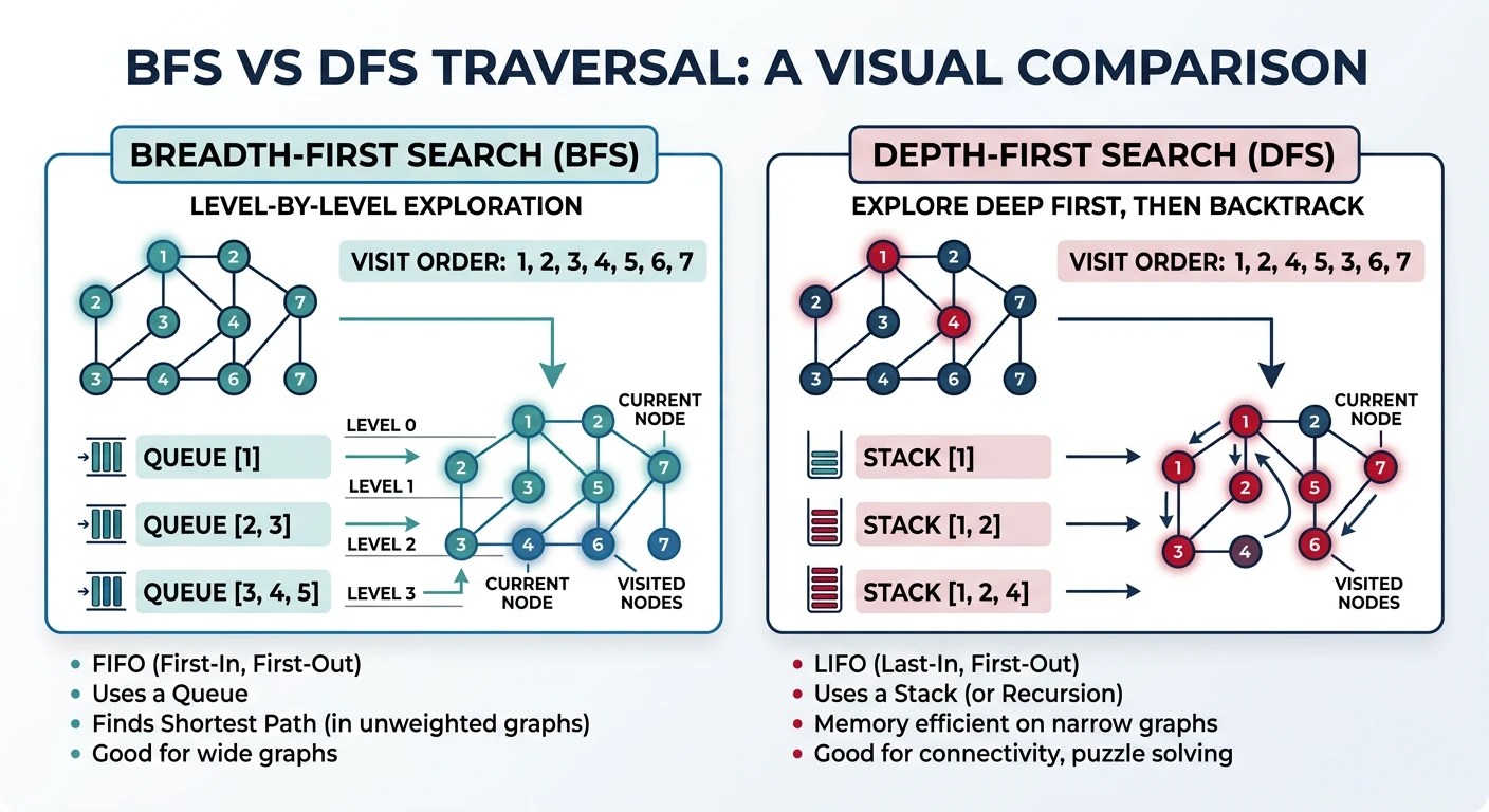
Step through both BFS and DFS on the same graph. Watch how the queue (BFS) explores level-by-level while the stack (DFS) dives deep before backtracking.

BFS vs DFS — Live Comparison

Unvisited Current In Queue/Stack Visited

BFS: Start at Node A

Click Next to step through BFS first, then DFS on the same graph.

Queue: [A] Step 1 / 10

Breadth-First Search (BFS)

BFS explores a graph level by level, visiting all neighbors at distance 1 before any at distance 2, and so on. It uses a queue (FIFO) to maintain the frontier. BFS naturally finds the shortest path in unweighted graphs because it discovers nodes in order of increasing distance from the source. Time: $O(V + E)$, Space: $O(V)$ for the visited set and queue.

When to use BFS: shortest path in unweighted graphs, level-order traversal, finding connected components, testing bipartiteness, or any problem where you need to explore "closest first" (like word ladder, minimum mutations, or maze shortest path).

from collections import deque, defaultdict

def bfs(graph, start):
    """
    Breadth-First Search
    Time: O(V + E), Space: O(V)
    Use for: shortest path in unweighted graphs, level-order traversal
    """
    visited = set([start])
    queue = deque([start])
    result = []

    while queue:
        node = queue.popleft()
        result.append(node)

        for neighbor in graph[node]:
            if neighbor not in visited:
                visited.add(neighbor)
                queue.append(neighbor)

    return result

def bfs_shortest_path(graph, start, end):
    """
    BFS for shortest path in unweighted graph
    Returns path from start to end
    """
    if start == end:
        return [start]

    visited = {start}
    queue = deque([(start, [start])])

    while queue:
        node, path = queue.popleft()

        for neighbor in graph[node]:
            if neighbor == end:
                return path + [neighbor]

            if neighbor not in visited:
                visited.add(neighbor)
                queue.append((neighbor, path + [neighbor]))

    return []  # No path found

# Example
graph = defaultdict(list)
edges = [(0, 1), (0, 2), (1, 2), (1, 3), (2, 3), (3, 4)]
for u, v in edges:
    graph[u].append(v)
    graph[v].append(u)

print("BFS traversal:", bfs(graph, 0))
print("Shortest path 0→4:", bfs_shortest_path(graph, 0, 4))

// BFS Traversal and Shortest Path
#include <vector>
#include <queue>
#include <unordered_set>
#include <unordered_map>

class GraphBFS {
public:
    // BFS traversal - O(V + E) time
    static std::vector<int> bfs(std::unordered_map<int, std::vector<int>>& graph, int start) {
        std::vector<int> result;
        std::unordered_set<int> visited;
        std::queue<int> q;

        visited.insert(start);
        q.push(start);

        while (!q.empty()) {
            int node = q.front(); q.pop();
            result.push_back(node);

            for (int neighbor : graph[node]) {
                if (visited.find(neighbor) == visited.end()) {
                    visited.insert(neighbor);
                    q.push(neighbor);
                }
            }
        }
        return result;
    }

    // Shortest path in unweighted graph
    static std::vector<int> shortestPath(std::unordered_map<int, std::vector<int>>& graph, int start, int end) {
        if (start == end) return {start};

        std::unordered_set<int> visited;
        std::queue<std::pair<int, std::vector<int>>> q;

        visited.insert(start);
        q.push({start, {start}});

        while (!q.empty()) {
            auto [node, path] = q.front(); q.pop();

            for (int neighbor : graph[node]) {
                if (neighbor == end) {
                    path.push_back(neighbor);
                    return path;
                }
                if (visited.find(neighbor) == visited.end()) {
                    visited.insert(neighbor);
                    std::vector<int> newPath = path;
                    newPath.push_back(neighbor);
                    q.push({neighbor, newPath});
                }
            }
        }
        return {};  // No path
    }
};

// BFS Traversal and Shortest Path
import java.util.*;

class GraphBFS {
    // BFS traversal - O(V + E) time
    public static List<Integer> bfs(Map<Integer, List<Integer>> graph, int start) {
        List<Integer> result = new ArrayList<>();
        Set<Integer> visited = new HashSet<>();
        Queue<Integer> queue = new LinkedList<>();

        visited.add(start);
        queue.offer(start);

        while (!queue.isEmpty()) {
            int node = queue.poll();
            result.add(node);

            for (int neighbor : graph.getOrDefault(node, new ArrayList<>())) {
                if (!visited.contains(neighbor)) {
                    visited.add(neighbor);
                    queue.offer(neighbor);
                }
            }
        }
        return result;
    }

    // Shortest path in unweighted graph
    public static List<Integer> shortestPath(Map<Integer, List<Integer>> graph, int start, int end) {
        if (start == end) return Arrays.asList(start);

        Set<Integer> visited = new HashSet<>();
        Queue<List<Integer>> queue = new LinkedList<>();

        visited.add(start);
        queue.offer(new ArrayList<>(Arrays.asList(start)));

        while (!queue.isEmpty()) {
            List<Integer> path = queue.poll();
            int node = path.get(path.size() - 1);

            for (int neighbor : graph.getOrDefault(node, new ArrayList<>())) {
                if (neighbor == end) {
                    path.add(neighbor);
                    return path;
                }
                if (!visited.contains(neighbor)) {
                    visited.add(neighbor);
                    List<Integer> newPath = new ArrayList<>(path);
                    newPath.add(neighbor);
                    queue.offer(newPath);
                }
            }
        }
        return new ArrayList<>();  // No path
    }
}

Depth-First Search (DFS)

DFS explores as deep as possible along each branch before backtracking. It uses a stack (explicit or via recursion's call stack). DFS is the natural choice for problems requiring exhaustive exploration: detecting cycles, topological sorting, finding connected/strongly-connected components, and solving puzzles (mazes, Sudoku). Time: $O(V + E)$, Space: $O(V)$ for the visited set plus $O(h)$ stack depth.

Recursive vs Iterative: Recursive DFS is cleaner for tree-like structures, but risks stack overflow on deep graphs (100K+ nodes). Iterative DFS with an explicit stack handles arbitrary depth safely.

from collections import defaultdict

def dfs_recursive(graph, start, visited=None):
    """
    DFS - Recursive implementation
    Time: O(V + E), Space: O(V) for call stack
    """
    if visited is None:
        visited = set()

    visited.add(start)
    result = [start]

    for neighbor in graph[start]:
        if neighbor not in visited:
            result.extend(dfs_recursive(graph, neighbor, visited))

    return result

def dfs_iterative(graph, start):
    """
    DFS - Iterative implementation using stack
    Time: O(V + E), Space: O(V)
    """
    visited = set()
    stack = [start]
    result = []

    while stack:
        node = stack.pop()

        if node not in visited:
            visited.add(node)
            result.append(node)

            # Add neighbors in reverse order for consistent ordering
            for neighbor in reversed(graph[node]):
                if neighbor not in visited:
                    stack.append(neighbor)

    return result

# Example
graph = defaultdict(list)
edges = [(0, 1), (0, 2), (1, 3), (1, 4), (2, 5)]
for u, v in edges:
    graph[u].append(v)
    graph[v].append(u)

print("DFS recursive:", dfs_recursive(graph, 0))
print("DFS iterative:", dfs_iterative(graph, 0))

// DFS Traversal - Recursive and Iterative
#include <vector>
#include <stack>
#include <unordered_set>
#include <unordered_map>

class GraphDFS {
public:
    // DFS recursive
    static std::vector<int> dfsRecursive(std::unordered_map<int, std::vector<int>>& graph,
                                          int node, std::unordered_set<int>& visited) {
        std::vector<int> result;
        visited.insert(node);
        result.push_back(node);

        for (int neighbor : graph[node]) {
            if (visited.find(neighbor) == visited.end()) {
                auto subResult = dfsRecursive(graph, neighbor, visited);
                result.insert(result.end(), subResult.begin(), subResult.end());
            }
        }
        return result;
    }

    // DFS iterative
    static std::vector<int> dfsIterative(std::unordered_map<int, std::vector<int>>& graph, int start) {
        std::vector<int> result;
        std::unordered_set<int> visited;
        std::stack<int> stk;

        stk.push(start);

        while (!stk.empty()) {
            int node = stk.top(); stk.pop();

            if (visited.find(node) == visited.end()) {
                visited.insert(node);
                result.push_back(node);

                // Add neighbors in reverse for consistent order
                auto& neighbors = graph[node];
                for (auto it = neighbors.rbegin(); it != neighbors.rend(); ++it) {
                    if (visited.find(*it) == visited.end())
                        stk.push(*it);
                }
            }
        }
        return result;
    }
};

// DFS Traversal - Recursive and Iterative
import java.util.*;

class GraphDFS {
    // DFS recursive
    public static void dfsRecursive(Map<Integer, List<Integer>> graph, int node,
                                     Set<Integer> visited, List<Integer> result) {
        visited.add(node);
        result.add(node);

        for (int neighbor : graph.getOrDefault(node, new ArrayList<>())) {
            if (!visited.contains(neighbor)) {
                dfsRecursive(graph, neighbor, visited, result);
            }
        }
    }

    // DFS iterative
    public static List<Integer> dfsIterative(Map<Integer, List<Integer>> graph, int start) {
        List<Integer> result = new ArrayList<>();
        Set<Integer> visited = new HashSet<>();
        Deque<Integer> stack = new ArrayDeque<>();

        stack.push(start);

        while (!stack.isEmpty()) {
            int node = stack.pop();

            if (!visited.contains(node)) {
                visited.add(node);
                result.add(node);

                List<Integer> neighbors = graph.getOrDefault(node, new ArrayList<>());
                for (int i = neighbors.size() - 1; i >= 0; i--) {
                    if (!visited.contains(neighbors.get(i)))
                        stack.push(neighbors.get(i));
                }
            }
        }
        return result;
    }
}

Number of Islands (Classic Graph Problem)

Given a 2D grid of '1's (land) and '0's (water), count the number of islands. An island is surrounded by water and formed by connecting adjacent lands horizontally or vertically. This is the canonical flood-fill / connected components problem: scan the grid; when you hit unvisited land, start a DFS/BFS to mark the entire island as visited, then increment the count. Each cell is visited at most once, giving $O(m \times n)$ time.

def num_islands(grid):
    """
    LeetCode 200: Number of Islands
    Time: O(m*n), Space: O(m*n) for recursion
    """
    if not grid:
        return 0

    rows, cols = len(grid), len(grid[0])
    count = 0

    def dfs(r, c):
        # Boundary check and water/visited check
        if (r < 0 or r >= rows or
            c < 0 or c >= cols or
            grid[r][c] != '1'):
            return

        # Mark as visited
        grid[r][c] = '#'

        # Explore all 4 directions
        dfs(r + 1, c)
        dfs(r - 1, c)
        dfs(r, c + 1)
        dfs(r, c - 1)

    for r in range(rows):
        for c in range(cols):
            if grid[r][c] == '1':
                count += 1
                dfs(r, c)

    return count

# Example
grid = [
    ['1', '1', '0', '0', '0'],
    ['1', '1', '0', '0', '0'],
    ['0', '0', '1', '0', '0'],
    ['0', '0', '0', '1', '1']
]

print("Number of islands:", num_islands(grid))  # 3

// LeetCode 200: Number of Islands
// Time: O(m*n), Space: O(m*n)
#include <vector>

class NumIslands {
public:
    int numIslands(std::vector<std::vector<char>>& grid) {
        if (grid.empty()) return 0;

        int rows = grid.size(), cols = grid[0].size();
        int count = 0;

        for (int r = 0; r < rows; r++) {
            for (int c = 0; c < cols; c++) {
                if (grid[r][c] == '1') {
                    count++;
                    dfs(grid, r, c, rows, cols);
                }
            }
        }
        return count;
    }

private:
    void dfs(std::vector<std::vector<char>>& grid, int r, int c, int rows, int cols) {
        if (r < 0 || r >= rows || c < 0 || c >= cols || grid[r][c] != '1')
            return;

        grid[r][c] = '#';  // Mark visited
        dfs(grid, r + 1, c, rows, cols);
        dfs(grid, r - 1, c, rows, cols);
        dfs(grid, r, c + 1, rows, cols);
        dfs(grid, r, c - 1, rows, cols);
    }
};

// LeetCode 200: Number of Islands
// Time: O(m*n), Space: O(m*n)

class NumIslands {
    public int numIslands(char[][] grid) {
        if (grid == null || grid.length == 0) return 0;

        int rows = grid.length, cols = grid[0].length;
        int count = 0;

        for (int r = 0; r < rows; r++) {
            for (int c = 0; c < cols; c++) {
                if (grid[r][c] == '1') {
                    count++;
                    dfs(grid, r, c, rows, cols);
                }
            }
        }
        return count;
    }

    private void dfs(char[][] grid, int r, int c, int rows, int cols) {
        if (r < 0 || r >= rows || c < 0 || c >= cols || grid[r][c] != '1')
            return;

        grid[r][c] = '#';  // Mark visited
        dfs(grid, r + 1, c, rows, cols);
        dfs(grid, r - 1, c, rows, cols);
        dfs(grid, r, c + 1, rows, cols);
        dfs(grid, r, c - 1, rows, cols);
    }
}

6. Exercises and Mastery

Easy

Given a raw edge list such as [(0,1), (0,2), (1,3)], build an adjacency list from it and print each vertex's neighbors.

Medium

Clone Graph (LeetCode 133): given a reference to a node in a connected undirected graph, return a deep copy of the entire graph. Use DFS or BFS with a hash map from original node to its clone to avoid infinite loops on cycles.

Hard

Given an undirected graph as an edge list, count the number of connected components. Run DFS or BFS from every unvisited vertex, incrementing a counter each time a traversal starts; the counter's final value is the component count.

Mastery challenge: A service ingests millions of user-to-user connection events and must answer "are these two users in the same friend network?" and "list every connection reachable from this user" with low latency. Choose a representation, justify it against the tradeoff table above, and explain how your traversal choice (BFS vs DFS) changes if the service also needs shortest number of hops between two users.

Review rhythm: tomorrow, redraw the three representations from memory for the same small graph and reconstruct their tradeoffs without notes; next week, implement BFS and DFS in all three languages without the code widgets open; several weeks later, solve Number of Islands and Clone Graph back to back and notice how both reduce to "traverse, mark visited, don't revisit."

7. Summary Cheat Sheet

A graph generalizes a tree: no required root, no required hierarchy, cycles allowed.
Adjacency List: $O(V+E)$ space, fast neighbor iteration, the default for sparse graphs.
Adjacency Matrix: $O(V^2)$ space, $O(1)$ edge existence check, best for dense graphs.
Edge List: $O(E)$ space, best when an algorithm must scan every edge; poor for BFS/DFS neighbor lookups.
BFS uses a queue and explores level by level; it finds shortest paths in unweighted graphs.
DFS uses a stack (explicit or via recursion) and explores as deep as possible before backtracking; it suits cycle detection, component counting, and exhaustive search.
Both BFS and DFS run in $O(V+E)$ time; a 2D grid (Number of Islands) is just a graph where neighbors are implicit.