Complete DSA Series Part 2: Recursion Complete Guide

FAANG Interview Prep

Your 12-step learning path • Currently on Step 2

Foundations, Memory & Complexity

Big-O notation, time/space analysis, memory layout

Recursion Complete Guide

Base cases, call stack, tail recursion, memoization

You Are Here

How Recursion Works

Recursion is a method where a function calls itself to solve a problem by breaking it down into smaller, similar subproblems. Every recursive solution needs two essential components.

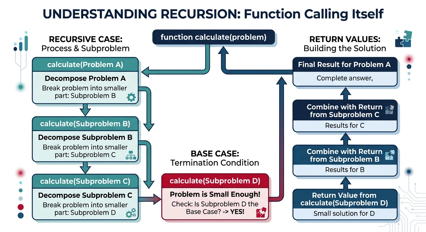
Recursion diagram showing a function calling itself with smaller subproblems until reaching the base case — How recursion works — a function calls itself with progressively smaller inputs until reaching the base case

                            Two Essential Components
                            Base Case: The condition that stops recursion (prevents infinite calls)
Recursive Case: The function calling itself with a modified input that moves toward the base case

                        

# Basic Recursion Structure
def factorial(n):
    # Base Case: Stop when n reaches 0 or 1
    if n <= 1:
        return 1
    
    # Recursive Case: n! = n × (n-1)!
    return n * factorial(n - 1)

# Test
print(f"5! = {factorial(5)}")  # Output: 120
print(f"0! = {factorial(0)}")  # Output: 1

// Basic Recursion Structure in C++
#include <iostream>
using namespace std;

int factorial(int n) {
    // Base Case: Stop when n reaches 0 or 1
    if (n <= 1) {
        return 1;
    }
    
    // Recursive Case: n! = n × (n-1)!
    return n * factorial(n - 1);
}

int main() {
    cout << "5! = " << factorial(5) << endl;  // Output: 120
    cout << "0! = " << factorial(0) << endl;  // Output: 1
    return 0;
}

// Basic Recursion Structure in Java
public class Factorial {
    // Recursive factorial method
    public static int factorial(int n) {
        // Base Case: Stop when n reaches 0 or 1
        if (n <= 1) {
            return 1;
        }
        
        // Recursive Case: n! = n × (n-1)!
        return n * factorial(n - 1);
    }
    
    public static void main(String[] args) {
        System.out.println("5! = " + factorial(5));  // Output: 120
        System.out.println("0! = " + factorial(0));  // Output: 1
    }
}

Call Stack Tracing

Understanding how the call stack works is crucial for mastering recursion. Each recursive call creates a new stack frame with its own local variables.

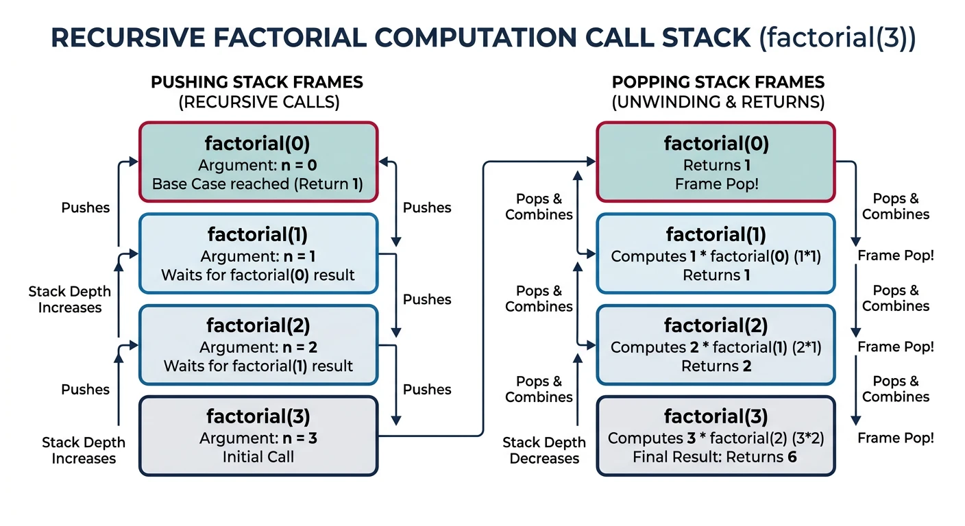
Call stack diagram showing stack frames pushed and popped during recursive factorial computation — Call stack during recursion — each call pushes a new stack frame; frames are popped as results return from base case upward

What is a Stack Frame?

Every time a function is called, a stack frame is pushed onto the call stack containing: the return address, function parameters, and local variables. When the function returns, its frame is popped off. In recursion, each call adds a new frame until the base case is reached, then frames are popped as results are returned.

# Visualizing Call Stack for factorial(4)

def factorial_traced(n, depth=0):
    """Factorial with call stack visualization"""
    indent = "  " * depth
    print(f"{indent}factorial({n}) called")
    
    if n <= 1:
        print(f"{indent}factorial({n}) returns 1 (base case)")
        return 1
    
    result = n * factorial_traced(n - 1, depth + 1)
    print(f"{indent}factorial({n}) returns {result}")
    return result

# Trace factorial(4)
print("Call Stack Trace:")
result = factorial_traced(4)
print(f"\nFinal Result: {result}")

# Output:
# factorial(4) called
#   factorial(3) called
#     factorial(2) called
#       factorial(1) called
#       factorial(1) returns 1 (base case)
#     factorial(2) returns 2
#   factorial(3) returns 6
# factorial(4) returns 24
# Final Result: 24

// Visualizing Call Stack for factorial(4) in C++
#include <iostream>
#include <string>
using namespace std;

int factorial_traced(int n, int depth = 0) {
    string indent(depth * 2, ' ');  // Create indentation
    cout << indent << "factorial(" << n << ") called" << endl;
    
    if (n <= 1) {
        cout << indent << "factorial(" << n << ") returns 1 (base case)" << endl;
        return 1;
    }
    
    int result = n * factorial_traced(n - 1, depth + 1);
    cout << indent << "factorial(" << n << ") returns " << result << endl;
    return result;
}

int main() {
    cout << "Call Stack Trace:" << endl;
    int result = factorial_traced(4);
    cout << "\nFinal Result: " << result << endl;
    return 0;
}

// Visualizing Call Stack for factorial(4) in Java
public class CallStackTrace {
    public static int factorialTraced(int n, int depth) {
        String indent = "  ".repeat(depth);  // Create indentation
        System.out.println(indent + "factorial(" + n + ") called");
        
        if (n <= 1) {
            System.out.println(indent + "factorial(" + n + ") returns 1 (base case)");
            return 1;
        }
        
        int result = n * factorialTraced(n - 1, depth + 1);
        System.out.println(indent + "factorial(" + n + ") returns " + result);
        return result;
    }
    
    public static void main(String[] args) {
        System.out.println("Call Stack Trace:");
        int result = factorialTraced(4, 0);
        System.out.println("\nFinal Result: " + result);
    }
}

Types of Recursion

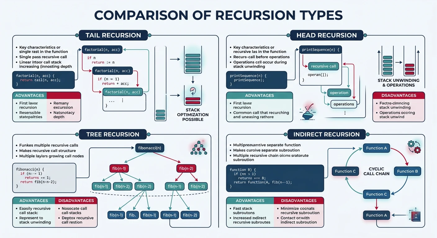
1. Tail Recursion

The recursive call is the last operation in the function. Can be optimized by compilers to use constant stack space (Tail Call Optimization).

Comparison of tail recursion, head recursion, tree recursion, and indirect recursion types — Types of recursion — tail, head, tree, and indirect recursion each differ in where and how recursive calls occur

Recursion Type Classification

graph TD
    R["Recursion"]
    R --> Direct["Direct Recursion"]
    R --> Indirect["Indirect Recursion"]

    Direct --> Linear["Linear
Single recursive call"]
    Direct --> Tail["Tail
Last operation is call"]
    Direct --> TreeR["Tree / Binary
Multiple recursive calls"]
    Direct --> Nested["Nested
Recursive arguments"]

    Indirect --> Mutual["Mutual
A calls B calls A"]

    style R fill:#132440,stroke:#132440,color:#fff
    style Direct fill:#16476A,stroke:#132440,color:#fff
    style Indirect fill:#3B9797,stroke:#132440,color:#fff

Why Tail Recursion Matters

In tail recursion, the recursive call is the absolute last operation in the function — there's no pending computation (like multiplication, addition, or concatenation) waiting for the result to come back. Because nothing needs to be remembered after the call, the compiler can replace the current stack frame instead of pushing a new one. This is called Tail Call Optimization (TCO), and it converts $O(n)$ stack space to $O(1)$ — effectively turning recursion into iteration under the hood.

Language support varies: Scheme and Haskell guarantee TCO by specification. JavaScript (ES6+) specifies it but only Safari implements it. C/C++ compilers (GCC, Clang) perform TCO at -O2 or higher as an optimization — not a guarantee. Java and Python never perform TCO by design (Python's Guido van Rossum explicitly rejected it to preserve readable stack traces). Understanding tail position helps you write recursion that can be optimized, and recognize when you must convert to iteration manually.

# Tail Recursion - recursive call is last operation
def factorial_tail(n, accumulator=1):
    """
    Tail-recursive factorial
    All computation done BEFORE the recursive call
    """
    if n <= 1:
        return accumulator
    return factorial_tail(n - 1, n * accumulator)  # Last operation

# Test
print(f"Tail recursive: {factorial_tail(5)}")  # Output: 120

// Tail Recursion in C++
#include <iostream>
using namespace std;

int factorial_tail(int n, int accumulator = 1) {
    // Base case
    if (n <= 1) {
        return accumulator;
    }
    // Tail recursive call - computation done before call
    return factorial_tail(n - 1, n * accumulator);
}

int main() {
    cout << "Tail recursive: " << factorial_tail(5) << endl;  // Output: 120
    return 0;
}

// Tail Recursion in Java
public class TailRecursion {
    public static int factorialTail(int n, int accumulator) {
        // Base case
        if (n <= 1) {
            return accumulator;
        }
        // Tail recursive call
        return factorialTail(n - 1, n * accumulator);
    }
    
    public static void main(String[] args) {
        System.out.println("Tail recursive: " + factorialTail(5, 1));  // Output: 120
    }
}

2. Head Recursion

The recursive call is made before any other processing. Work is done during the "unwinding" phase.

# Head Recursion - processing after recursive call
def print_numbers_head(n):
    """
    Head-recursive: prints numbers 1 to n
    Processing happens AFTER the recursive call returns
    """
    if n == 0:
        return
    print_numbers_head(n - 1)  # Recursive call FIRST
    print(n)  # Processing AFTER

# Test
print("Head Recursion (1 to 5):")
print_numbers_head(5)  # Output: 1, 2, 3, 4, 5

// Head Recursion in C++
#include <iostream>
using namespace std;

void printNumbersHead(int n) {
    if (n == 0) {
        return;
    }
    printNumbersHead(n - 1);  // Recursive call FIRST
    cout << n << " ";         // Processing AFTER
}

int main() {
    cout << "Head Recursion (1 to 5): ";
    printNumbersHead(5);  // Output: 1 2 3 4 5
    cout << endl;
    return 0;
}

// Head Recursion in Java
public class HeadRecursion {
    public static void printNumbersHead(int n) {
        if (n == 0) {
            return;
        }
        printNumbersHead(n - 1);  // Recursive call FIRST
        System.out.print(n + " ");  // Processing AFTER
    }
    
    public static void main(String[] args) {
        System.out.print("Head Recursion (1 to 5): ");
        printNumbersHead(5);  // Output: 1 2 3 4 5
        System.out.println();
    }
}

3. Tree Recursion

The function makes multiple recursive calls in each invocation, creating a tree-like call structure.

Warning: Exponential Growth

Tree recursion often leads to exponential time complexity O(2n) because each call spawns multiple new calls. For Fibonacci, fib(40) makes over 300 million function calls! Always consider memoization or iterative solutions for tree recursive problems.

# Tree Recursion - multiple recursive calls
def fibonacci_tree(n):
    """
    Tree-recursive Fibonacci
    Each call branches into two more calls
    Time: O(2^n) - exponential!
    """
    if n <= 1:
        return n
    return fibonacci_tree(n - 1) + fibonacci_tree(n - 2)  # Two calls

# Test
print(f"Fibonacci(10) = {fibonacci_tree(10)}")  # Output: 55

// Tree Recursion in C++
#include <iostream>
using namespace std;

int fibonacci_tree(int n) {
    // Base case
    if (n <= 1) {
        return n;
    }
    // Tree recursion - two recursive calls
    return fibonacci_tree(n - 1) + fibonacci_tree(n - 2);
}

int main() {
    cout << "Fibonacci(10) = " << fibonacci_tree(10) << endl;  // Output: 55
    return 0;
}

// Tree Recursion in Java
public class TreeRecursion {
    public static int fibonacciTree(int n) {
        // Base case
        if (n <= 1) {
            return n;
        }
        // Tree recursion - two recursive calls
        return fibonacciTree(n - 1) + fibonacciTree(n - 2);
    }
    
    public static void main(String[] args) {
        System.out.println("Fibonacci(10) = " + fibonacciTree(10));  // Output: 55
    }
}

4. Indirect Recursion

Function A calls function B, which calls function A (or through more functions in a cycle).

# Indirect Recursion - functions call each other
def is_even(n):
    if n == 0:
        return True
    return is_odd(n - 1)

def is_odd(n):
    if n == 0:
        return False
    return is_even(n - 1)

# Test
print(f"is_even(4) = {is_even(4)}")  # True
print(f"is_odd(5) = {is_odd(5)}")    # True

// Indirect Recursion in C++
#include <iostream>
using namespace std;

// Forward declaration needed for indirect recursion
bool isOdd(int n);

bool isEven(int n) {
    if (n == 0) return true;
    return isOdd(n - 1);
}

bool isOdd(int n) {
    if (n == 0) return false;
    return isEven(n - 1);
}

int main() {
    cout << "isEven(4) = " << (isEven(4) ? "true" : "false") << endl;  // true
    cout << "isOdd(5) = " << (isOdd(5) ? "true" : "false") << endl;    // true
    return 0;
}

// Indirect Recursion in Java
public class IndirectRecursion {
    public static boolean isEven(int n) {
        if (n == 0) return true;
        return isOdd(n - 1);
    }
    
    public static boolean isOdd(int n) {
        if (n == 0) return false;
        return isEven(n - 1);
    }
    
    public static void main(String[] args) {
        System.out.println("isEven(4) = " + isEven(4));  // true
        System.out.println("isOdd(5) = " + isOdd(5));    // true
    }
}

5. Nested Recursion

A recursive call is used as an argument to another recursive call.

The Ackermann Function

The Ackermann function $A(m, n)$ is named after German mathematician Wilhelm Ackermann. It is one of the earliest discovered examples of a total computable function that is not primitive recursive — meaning it can be solved by a computer program, but grows so unimaginably fast that it cannot be computed using basic loops where the number of iterations is known in advance. It requires deep recursion.

The function is defined for two non-negative integers using three rules:

$$A(m, n) = \begin{cases} n + 1 & \text{if } m = 0 \\ A(m - 1, 1) & \text{if } m > 0 \text{ and } n = 0 \\ A(m - 1, A(m, n - 1)) & \text{if } m > 0 \text{ and } n > 0 \end{cases}$$

The third rule — $A(m - 1, \mathbf{A(m, n - 1)})$ — is the key: the function calls itself, then uses that result as input for another call to itself. This nested recursion drives its explosive growth.

How Fast Does It Grow?

$m$	Growth Pattern	Example
0	Linear: $n + 1$	$A(0, 5) = 6$
1	Addition: $n + 2$	$A(1, 5) = 7$
2	Multiplication: $2n + 3$	$A(2, 5) = 13$
3	Exponentiation: $2^{n+3} - 3$	$A(3, 5) = 253$
4	Tetration (tower of exponents)	$A(4, 2) = 2^{65536} - 3$ (19,729 digits!)

$A(4, 2)$ already exceeds the number of atoms in the observable universe. Attempting $A(4, 3)$ would overflow any call stack almost instantly.

Why Computer Scientists Care

Stress-testing compilers: Even tiny inputs like $A(4, 1)$ generate a massive number of function calls, making it ideal for benchmarking how well a compiler optimizes recursive calls and manages stack memory.

Algorithm analysis: The inverse Ackermann function $\alpha(n)$ grows incredibly slowly and appears in the time complexity of the Disjoint-Set (Union-Find) data structure. For all practical input sizes, $\alpha(n) \leq 4$, making Union-Find operations effectively $O(1)$ amortized — a result we'll explore in Part 13: Advanced Structures.

# Nested Recursion - recursive call as argument
def ackermann(m, n):
    """
    Ackermann function - classic nested recursion example
    Grows EXTREMELY fast
    """
    if m == 0:
        return n + 1
    if n == 0:
        return ackermann(m - 1, 1)
    return ackermann(m - 1, ackermann(m, n - 1))  # Nested!

# Test (only small values!)
print(f"ackermann(2, 2) = {ackermann(2, 2)}")  # Output: 7
print(f"ackermann(3, 2) = {ackermann(3, 2)}")  # Output: 29

// Nested Recursion - Ackermann Function in C++
#include <iostream>
using namespace std;

int ackermann(int m, int n) {
    if (m == 0) {
        return n + 1;
    }
    if (n == 0) {
        return ackermann(m - 1, 1);
    }
    // Nested recursion - inner call's result becomes argument
    return ackermann(m - 1, ackermann(m, n - 1));
}

int main() {
    cout << "ackermann(2, 2) = " << ackermann(2, 2) << endl;  // Output: 7
    cout << "ackermann(3, 2) = " << ackermann(3, 2) << endl;  // Output: 29
    return 0;
}

// Nested Recursion - Ackermann Function in Java
public class NestedRecursion {
    public static int ackermann(int m, int n) {
        if (m == 0) {
            return n + 1;
        }
        if (n == 0) {
            return ackermann(m - 1, 1);
        }
        // Nested recursion - inner call's result becomes argument
        return ackermann(m - 1, ackermann(m, n - 1));
    }
    
    public static void main(String[] args) {
        System.out.println("ackermann(2, 2) = " + ackermann(2, 2));  // Output: 7
        System.out.println("ackermann(3, 2) = " + ackermann(3, 2));  // Output: 29
    }
}

Recurrence Relations

What is a Recurrence Relation?

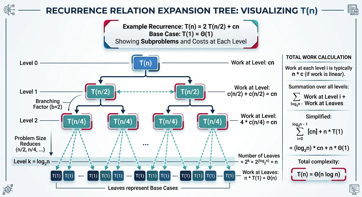
A recurrence relation is a mathematical equation that defines a sequence where each term is expressed in terms of preceding terms. In algorithm analysis, we use recurrence relations to describe the time complexity of recursive algorithms.

General form: $T(n)$ = [number of subproblems] × T([subproblem size]) + [work done outside recursive calls]

Breaking Down a Recurrence

Consider Merge Sort's recurrence: $T(n) = 2T(n/2) + O(n)$

2 = number of subproblems (we split into two halves)
$T(n/2)$ = each subproblem is half the size
$O(n)$ = work to merge the two halves back together

Understanding how to write and solve these equations is crucial for analyzing recursive algorithms!

Common Recurrence Patterns

Here are the most frequently encountered recurrence patterns in algorithm analysis:

Recurrence relation expansion tree showing how $T(n)$ breaks into subproblems at each level — Recurrence relation expansion — visualizing how $T(n)$ decomposes into subproblems at each recursive level

Pattern Reference Table

Recurrence	Result	Example Algorithm	Explanation
$T(n) = T(n-1) + O(1)$	$O(n)$	Factorial, Linear Search	Constant work, $n$ calls deep
$T(n) = T(n-1) + O(n)$	$O(n^{2})$	Selection Sort (recursive)	$n + (n-1) + \cdots + 1 = \frac{n(n+1)}{2}$
$T(n) = 2T(n/2) + O(n)$	$O(n \log n)$	Merge Sort, Quick Sort (avg)	$n$ work at each of $\log n$ levels
$T(n) = 2T(n/2) + O(1)$	$O(n)$	Binary tree traversal	Visit each of $n$ nodes once
$T(n) = T(n/2) + O(1)$	$O(\log n)$	Binary Search	Halve problem each step
$T(n) = T(n/2) + O(n)$	$O(n)$	Finding median	$n + n/2 + n/4 + \cdots = 2n$
$T(n) = 2T(n-1) + O(1)$	$O(2^n)$	Naive Fibonacci, Tower of Hanoi	Exponential — avoid if possible!
$T(n) = T(n-1) + T(n-2)$	$O(\phi^n)$	Fibonacci ($\phi \approx 1.618$)	Golden ratio growth

Solving Recurrences: Step-by-Step Example

Let's solve $T(n) = 2T(n/2) + n$ using the substitution method (repeated expansion):

Step 1: Expand the Recurrence (Unroll It)

$$T(n) = 2T\!\left(\frac{n}{2}\right) + n$$

Substitute $T(n/2) = 2T(n/4) + n/2$:

$$T(n) = 2\left[2T\!\left(\frac{n}{4}\right) + \frac{n}{2}\right] + n = 4T\!\left(\frac{n}{4}\right) + 2n$$

Substitute again:

$$T(n) = 4\left[2T\!\left(\frac{n}{8}\right) + \frac{n}{4}\right] + 2n = 8T\!\left(\frac{n}{8}\right) + 3n$$

Step 2: Find the Pattern

After $k$ iterations:

$$T(n) = 2^k \cdot T\!\left(\frac{n}{2^k}\right) + k \cdot n$$

Step 3: Find When to Stop (Base Case)

Recursion stops when the subproblem hits the base case $T(1)$:

$$\frac{n}{2^k} = 1 \implies 2^k = n \implies k = \log_2 n$$

Step 4: Substitute Back

Replace $k = \log_2 n$ and $2^k = n$:

$$T(n) = n \cdot T(1) + n \cdot \log_2 n = n \cdot O(1) + n \log n$$

$$\boxed{T(n) = O(n \log n)}$$

Master Theorem

The Power of the Master Theorem

The Master Theorem is a "cookbook" method that lets you instantly determine the complexity of many divide-and-conquer algorithms without manual expansion. It works for recurrences of this form:

$$T(n) = a \cdot T\!\left(\frac{n}{b}\right) + f(n)$$

Where:

$a \geq 1$ = number of subproblems
$b > 1$ = factor by which input size is divided
$f(n)$ = cost of work done outside the recursive calls

The Three Cases

Let $c_{\text{crit}} = \log_b a$ (the critical exponent). Compare $f(n)$ to $n^{c_{\text{crit}}}$:

Case	Condition	Result	Intuition
1	$f(n) = O(n^c)$ where $c < \log_b a$	$T(n) = \Theta(n^{\log_b a})$	Recursion dominates
2	$f(n) = \Theta(n^{\log_b a})$	$T(n) = \Theta(n^{\log_b a} \log n)$	Work is evenly distributed
3	$f(n) = \Omega(n^c)$ where $c > \log_b a$	$T(n) = \Theta(f(n))$	Non-recursive work dominates

Master Theorem Examples

Example 1 Merge Sort: $T(n) = 2T(n/2) + O(n)$

$a = 2$ (two subproblems), $b = 2$ (each is half the size)
$f(n) = n$ (merging takes linear time)
$\log_b a = \log_2 2 = 1$
$f(n) = n = \Theta(n^1) = \Theta(n^{\log_b a})$ → Case 2!

$$\boxed{T(n) = \Theta(n \log n)}$$

Example 2 Binary Search: $T(n) = T(n/2) + O(1)$

$a = 1$ (one subproblem), $b = 2$ (half the size)
$f(n) = 1$ (constant comparison)
$\log_b a = \log_2 1 = 0$
$f(n) = 1 = \Theta(n^0) = \Theta(n^{\log_b a})$ → Case 2!

$$\boxed{T(n) = \Theta(\log n)}$$

Example 3 Karatsuba Multiplication: $T(n) = 3T(n/2) + O(n)$

$a = 3$, $b = 2$, $f(n) = n$
$\log_b a = \log_2 3 \approx 1.585$
$f(n) = n = O(n^1)$, and $1 < 1.585$ → Case 1!

$$\boxed{T(n) = \Theta(n^{\log_2 3}) \approx O(n^{1.585})}$$

Better than the naive $O(n^2)$ multiplication!

Example 4 Strassen's Matrix Multiplication: $T(n) = 7T(n/2) + O(n^{2})$

$a = 7$, $b = 2$, $f(n) = n^2$
$\log_b a = \log_2 7 \approx 2.807$
$f(n) = n^2 = O(n^2)$, and $2 < 2.807$ → Case 1!

$$\boxed{T(n) = \Theta(n^{\log_2 7}) \approx O(n^{2.807})}$$

Better than naive $O(n^3)$ matrix multiplication!

When Master Theorem Doesn't Apply

The Master Theorem has limitations. It doesn't work for:

Non-constant subproblem sizes: $T(n) = T(n/2) + T(n/3) + n$
Subtract recurrences: $T(n) = T(n-1) + n$ (use substitution instead)
Non-polynomial f(n): $T(n) = 2T(n/2) + n \log n$ (special case, use extended theorem)
a < 1 or b = 1 (violates theorem prerequisites)

For these cases, use the substitution method or recursion tree method.

Classic Recursive Problems

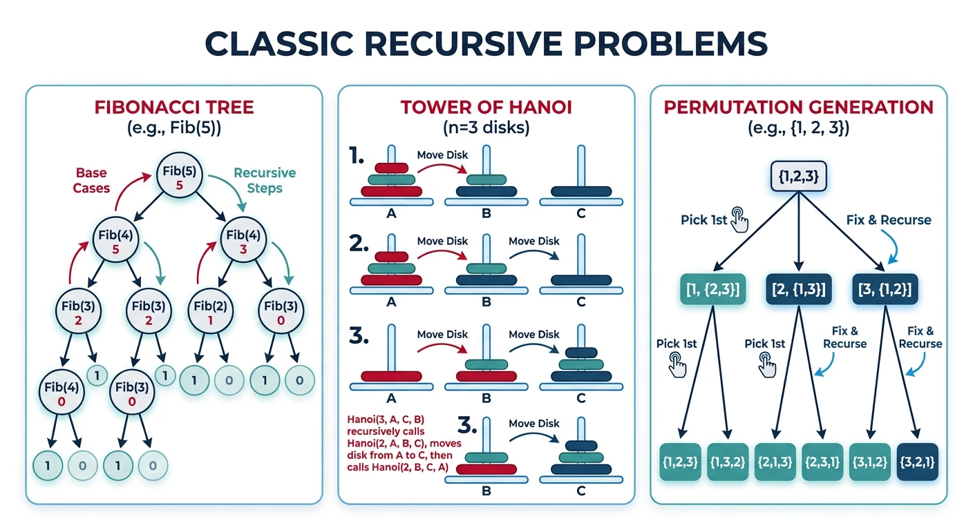
Fibonacci Sequence

The Fibonacci Story

The Fibonacci sequence was introduced to Western mathematics by Italian mathematician Leonardo of Pisa (nicknamed Fibonacci) in his 1202 book "Liber Abaci". He used it to model rabbit population growth:

Month 1: Start with 1 pair of rabbits
Month 2: Still 1 pair (too young to reproduce)
Month 3: 2 pairs (original pair has 1 offspring)
Month 4: 3 pairs (original pair has another offspring)
Month 5: 5 pairs, Month 6: 8 pairs, and so on...

The sequence: 0, 1, 1, 2, 3, 5, 8, 13, 21, 34, 55, 89, 144... where each number is the sum of the two preceding ones.

Mathematical Definition

The Fibonacci sequence is defined recursively as:

$$F(n) = \begin{cases} 0 & \text{if } n = 0 \\ 1 & \text{if } n = 1 \\ F(n-1) + F(n-2) & \text{if } n \geq 2 \end{cases}$$

This naturally leads to a recursive solution, but the naive approach has exponential time complexity $O(\phi^n)$ where $\phi = \frac{1+\sqrt{5}}{2} \approx 1.618$ (the golden ratio), due to repeated calculations. We'll explore three approaches to optimize it.

Approach 1: Naive Tree Recursion - $O(2^{n})$

The simplest implementation directly follows the mathematical definition, but it's extremely inefficient because it recalculates the same values many times:

                    fib(5)
                   /      \
              fib(4)      fib(3)
             /    \        /    \
         fib(3)  fib(2)  fib(2)  fib(1)
         /   \    /   \    /   \
     fib(2) fib(1) ...  ...  ...

Notice how fib(3) is calculated twice, fib(2) is calculated 3 times!
This exponential growth makes naive recursion impractical for n > 40.

# Fibonacci - Naive Tree Recursion
# Time Complexity: O(2^n) - exponential
# Space Complexity: O(n) - recursion stack depth

def fib_naive(n):
    """Calculate nth Fibonacci number using naive recursion."""
    # Base cases
    if n <= 1:
        return n
    # Recursive case: F(n) = F(n-1) + F(n-2)
    return fib_naive(n - 1) + fib_naive(n - 2)

# Test - only works reasonably for small n
for i in range(11):
    print(f"F({i}) = {fib_naive(i)}")
# Output: 0, 1, 1, 2, 3, 5, 8, 13, 21, 34, 55

#include <iostream>
using namespace std;

// Naive Tree Recursion - O(2^n) time
int fib_naive(int n) {
    // Base cases
    if (n <= 1) {
        return n;
    }
    // Recursive case
    return fib_naive(n - 1) + fib_naive(n - 2);
}

int main() {
    cout << "Fibonacci Sequence (Naive):" << endl;
    for (int i = 0; i <= 10; i++) {
        cout << "F(" << i << ") = " << fib_naive(i) << endl;
    }
    // Output: 0, 1, 1, 2, 3, 5, 8, 13, 21, 34, 55
    return 0;
}

public class FibonacciNaive {
    // Naive Tree Recursion - O(2^n) time
    public static int fibNaive(int n) {
        // Base cases
        if (n <= 1) {
            return n;
        }
        // Recursive case
        return fibNaive(n - 1) + fibNaive(n - 2);
    }
    
    public static void main(String[] args) {
        System.out.println("Fibonacci Sequence (Naive):");
        for (int i = 0; i <= 10; i++) {
            System.out.println("F(" + i + ") = " + fibNaive(i));
        }
        // Output: 0, 1, 1, 2, 3, 5, 8, 13, 21, 34, 55
    }
}

Approach 2: Memoization (Top-Down DP) - $O(n)$

We can dramatically improve performance by storing already-computed values in a cache (memo). This technique is called memoization and is the foundation of Dynamic Programming:

# Fibonacci - Memoization (Top-Down DP)
# Time Complexity: O(n) - each value computed once
# Space Complexity: O(n) - memo dictionary + recursion stack

def fib_memo(n, memo=None):
    """Calculate nth Fibonacci with memoization."""
    if memo is None:
        memo = {}
    
    # Check if already computed
    if n in memo:
        return memo[n]
    
    # Base cases
    if n <= 1:
        return n
    
    # Compute and store in memo
    memo[n] = fib_memo(n - 1, memo) + fib_memo(n - 2, memo)
    return memo[n]

# Now we can calculate much larger values efficiently!
print(f"F(50) = {fib_memo(50)}")   # 12586269025
print(f"F(100) = {fib_memo(100)}") # 354224848179261915075

#include <iostream>
#include <unordered_map>
using namespace std;

// Memoization using hash map - O(n) time
unordered_map<int, long long> memo;

long long fib_memo(int n) {
    // Check if already computed
    if (memo.find(n) != memo.end()) {
        return memo[n];
    }
    
    // Base cases
    if (n <= 1) {
        return n;
    }
    
    // Compute and store in memo
    memo[n] = fib_memo(n - 1) + fib_memo(n - 2);
    return memo[n];
}

int main() {
    cout << "Fibonacci with Memoization:" << endl;
    cout << "F(50) = " << fib_memo(50) << endl;  // 12586269025
    
    // Reset memo for clean test
    memo.clear();
    for (int i = 0; i <= 15; i++) {
        cout << "F(" << i << ") = " << fib_memo(i) << endl;
    }
    return 0;
}

import java.util.HashMap;
import java.util.Map;

public class FibonacciMemo {
    // Use HashMap for memoization
    private static Map<Integer, Long> memo = new HashMap<>();
    
    public static long fibMemo(int n) {
        // Check if already computed
        if (memo.containsKey(n)) {
            return memo.get(n);
        }
        
        // Base cases
        if (n <= 1) {
            return n;
        }
        
        // Compute and store in memo
        long result = fibMemo(n - 1) + fibMemo(n - 2);
        memo.put(n, result);
        return result;
    }
    
    public static void main(String[] args) {
        System.out.println("Fibonacci with Memoization:");
        System.out.println("F(50) = " + fibMemo(50));  // 12586269025
        
        // Print sequence
        memo.clear();
        for (int i = 0; i <= 15; i++) {
            System.out.println("F(" + i + ") = " + fibMemo(i));
        }
    }
}

Approach 3: Iterative (Bottom-Up DP) - $O(n)$ time, $O(1)$ space

The most efficient approach uses iteration instead of recursion. We only need to track the last two values, reducing space complexity to $O(1)$:

# Fibonacci - Iterative (Bottom-Up DP)
# Time Complexity: O(n)
# Space Complexity: O(1) - only two variables!

def fib_iterative(n):
    """Calculate nth Fibonacci iteratively - most efficient!"""
    if n <= 1:
        return n
    
    # Only track the last two values
    prev2, prev1 = 0, 1  # F(0), F(1)
    
    for i in range(2, n + 1):
        current = prev1 + prev2
        prev2 = prev1
        prev1 = current
    
    return prev1

# Test all three approaches
print("Iterative approach (O(1) space):")
print(f"F(50) = {fib_iterative(50)}")   # 12586269025
print(f"F(100) = {fib_iterative(100)}") # 354224848179261915075

#include <iostream>
using namespace std;

// Iterative approach - O(n) time, O(1) space
long long fib_iterative(int n) {
    if (n <= 1) {
        return n;
    }
    
    // Only track the last two values
    long long prev2 = 0, prev1 = 1;
    
    for (int i = 2; i <= n; i++) {
        long long current = prev1 + prev2;
        prev2 = prev1;
        prev1 = current;
    }
    
    return prev1;
}

int main() {
    cout << "Fibonacci Iterative (O(1) space):" << endl;
    cout << "F(50) = " << fib_iterative(50) << endl;  // 12586269025
    
    // Print sequence
    for (int i = 0; i <= 15; i++) {
        cout << "F(" << i << ") = " << fib_iterative(i) << endl;
    }
    return 0;
}

public class FibonacciIterative {
    // Iterative approach - O(n) time, O(1) space
    public static long fibIterative(int n) {
        if (n <= 1) {
            return n;
        }
        
        // Only track the last two values
        long prev2 = 0, prev1 = 1;
        
        for (int i = 2; i <= n; i++) {
            long current = prev1 + prev2;
            prev2 = prev1;
            prev1 = current;
        }
        
        return prev1;
    }
    
    public static void main(String[] args) {
        System.out.println("Fibonacci Iterative (O(1) space):");
        System.out.println("F(50) = " + fibIterative(50));  // 12586269025
        
        // Print sequence
        for (int i = 0; i <= 15; i++) {
            System.out.println("F(" + i + ") = " + fibIterative(i));
        }
    }
}

                            Complexity Comparison
                            
                                        Approach
                                        Time
                                        Space
                                        When to Use
                                    
                                        Naive Recursion
                                        \(O(2^{n})\)
                                        \(O(n)\)
                                        Only for teaching purposes
                                    
                                        Memoization
                                        \(O(n)\)
                                        \(O(n)\)
                                        When you need recursion structure
                                    
                                        Iterative
                                        \(O(n)\)
                                        \(O(1)\)
                                        Best for production code

Approach	Time	Space	When to Use
Naive Recursion	\(O(2^{n})\)	\(O(n)\)	Only for teaching purposes
Memoization	\(O(n)\)	\(O(n)\)	When you need recursion structure
Iterative	\(O(n)\)	\(O(1)\)	Best for production code

Tower of Hanoi

The Legend

The Tower of Hanoi is a mathematical puzzle invented by French mathematician Édouard Lucas in 1883. Legend has it that in a temple in Hanoi, monks have been moving 64 golden disks between three diamond pegs since the beginning of time. When they finish, the world will end!

Fun fact: With 64 disks, it would take $2^{64} - 1 \approx 1.84 \times 10^{19}$ moves. At one move per second, that's about 585 billion years!

Problem Statement

You have 3 pegs (rods) labeled A, B, and C. Peg A has n disks stacked in decreasing size (largest at bottom). Goal: Move all disks from A to C.

Rules:
1. Only one disk can be moved at a time
2. Each move takes the top disk from one peg and places it on another
3. No disk may be placed on top of a smaller disk

The Recursive Insight

The key insight is to think recursively: to move n disks from A to C, we need to:

Move n-1 disks from A to B (using C as helper)
Move the largest disk from A to C
Move n-1 disks from B to C (using A as helper)

Visual Trace for 3 Disks

Initial State:          After Move 1:           After Move 2:
    |     |     |           |     |     |           |     |     |
   [1]    |     |           |     |     |          [1]    |     |
   [2]    |     |          [2]    |     |          [2]    |     |
   [3]    |     |          [3]   [1]    |          [3]   [1]    |
  -----  -----  -----     -----  -----  -----     -----  -----  -----
    A      B      C           A      B      C         A      B      C

After Move 3:           After Move 4:           After Move 5:
    |     |     |           |     |     |           |     |     |
    |     |     |           |     |     |           |     |    [1]
   [2]    |     |           |     |     |           |     |    [2]
   [3]   [1]   [2]          |    [1]   [2]          |    [1]   [2]
  -----  -----  -----     -----  -----  -----     -----  -----  -----
    A      B      C           A      B      C         A      B      C

After Move 6:           After Move 7 (DONE!):
    |     |     |           |     |     |
    |     |    [1]          |     |    [1]
    |     |    [2]          |     |    [2]
   [3]    |     |          [3]    |    [3]
  -----  -----  -----     -----  -----  -----
    A      B      C           A      B      C

The 7 moves: (2^3 - 1 = 7)
1. Move disk 1 from A to C
2. Move disk 2 from A to B
3. Move disk 1 from C to B
4. Move disk 3 from A to C  ? The crucial "middle" move
5. Move disk 1 from B to A
6. Move disk 2 from B to C
7. Move disk 1 from A to C

# Tower of Hanoi - Classic Recursion Problem
def tower_of_hanoi(n, source, auxiliary, destination):
    """
    Solve Tower of Hanoi for n disks
    Time Complexity: O(2^n) - must make 2^n - 1 moves
    Space Complexity: O(n) - recursion depth
    """
    if n == 1:
        print(f"Move disk 1 from {source} to {destination}")
        return
    
    # Step 1: Move n-1 disks from source to auxiliary (using destination as helper)
    tower_of_hanoi(n - 1, source, destination, auxiliary)
    
    # Step 2: Move the largest disk from source to destination
    print(f"Move disk {n} from {source} to {destination}")
    
    # Step 3: Move n-1 disks from auxiliary to destination (using source as helper)
    tower_of_hanoi(n - 1, auxiliary, source, destination)

# Test with 3 disks
print("Tower of Hanoi with 3 disks:")
tower_of_hanoi(3, 'A', 'B', 'C')
print(f"\nTotal moves for n disks: 2^n - 1 = {2**3 - 1} moves")

// Tower of Hanoi in C++
#include <iostream>
#include <string>
using namespace std;

void towerOfHanoi(int n, char source, char auxiliary, char destination) {
    // Base case: only one disk
    if (n == 1) {
        cout << "Move disk 1 from " << source << " to " << destination << endl;
        return;
    }
    
    // Step 1: Move n-1 disks from source to auxiliary
    towerOfHanoi(n - 1, source, destination, auxiliary);
    
    // Step 2: Move largest disk from source to destination
    cout << "Move disk " << n << " from " << source << " to " << destination << endl;
    
    // Step 3: Move n-1 disks from auxiliary to destination
    towerOfHanoi(n - 1, auxiliary, source, destination);
}

int main() {
    int n = 3;
    cout << "Tower of Hanoi with " << n << " disks:" << endl;
    towerOfHanoi(n, 'A', 'B', 'C');
    cout << "\nTotal moves: " << (1 << n) - 1 << endl;  // 2^n - 1
    return 0;
}

// Tower of Hanoi in Java
public class TowerOfHanoi {
    public static void towerOfHanoi(int n, char source, char auxiliary, char destination) {
        // Base case: only one disk
        if (n == 1) {
            System.out.println("Move disk 1 from " + source + " to " + destination);
            return;
        }
        
        // Step 1: Move n-1 disks from source to auxiliary
        towerOfHanoi(n - 1, source, destination, auxiliary);
        
        // Step 2: Move largest disk from source to destination
        System.out.println("Move disk " + n + " from " + source + " to " + destination);
        
        // Step 3: Move n-1 disks from auxiliary to destination
        towerOfHanoi(n - 1, auxiliary, source, destination);
    }
    
    public static void main(String[] args) {
        int n = 3;
        System.out.println("Tower of Hanoi with " + n + " disks:");
        towerOfHanoi(n, 'A', 'B', 'C');
        System.out.println("\nTotal moves: " + ((1 << n) - 1));  // 2^n - 1
    }
}

Tower of Hanoi Complexity Analysis

Recurrence Relation: $T(n)$ = 2T(n-1) + 1

Solving:

T(1) = 1
T(2) = 2(1) + 1 = 3
T(3) = 2(3) + 1 = 7
$T(n)$ = 2n - 1

Time Complexity: O(2n) — exponential, unavoidable for this problem
Space Complexity: $O(n)$ — recursion stack depth

Power Function

The Exponentiation Problem

Computing $x^n$ is a fundamental operation in mathematics and computing. While we could simply multiply $x$ by itself $n$ times ($O(n)$ time), there's a brilliant technique called exponentiation by squaring that reduces this to $O(\log n)$!

Key insight: $x^8 = ((x^2)^2)^2$ — only 3 multiplications instead of 7!

Mathematical Basis

Exponentiation by squaring exploits two properties:

Even exponent: $x^n = (x^{n/2})^2$
Odd exponent: $x^n = x \cdot x^{n-1}$

This halves the problem size at each step, giving us $O(\log n)$ time complexity!

Approach 1: Naive Recursion - $O(n)$

The straightforward approach multiplies the base n times:

# Power Function - Naive Recursion
# Time Complexity: O(n) - makes n recursive calls
# Space Complexity: O(n) - recursion stack depth

def power_naive(base, exp):
    """Calculate base^exp using naive recursion."""
    # Base case: x^0 = 1
    if exp == 0:
        return 1
    # Recursive case: x^n = x * x^(n-1)
    return base * power_naive(base, exp - 1)

# Test
print(f"2^10 = {power_naive(2, 10)}")  # 1024
print(f"3^5 = {power_naive(3, 5)}")    # 243

#include <iostream>
using namespace std;

// Naive recursion - O(n) time
long long power_naive(int base, int exp) {
    // Base case: x^0 = 1
    if (exp == 0) {
        return 1;
    }
    // Recursive case: x^n = x * x^(n-1)
    return base * power_naive(base, exp - 1);
}

int main() {
    cout << "2^10 = " << power_naive(2, 10) << endl;  // 1024
    cout << "3^5 = " << power_naive(3, 5) << endl;    // 243
    return 0;
}

public class PowerNaive {
    // Naive recursion - O(n) time
    public static long powerNaive(int base, int exp) {
        // Base case: x^0 = 1
        if (exp == 0) {
            return 1;
        }
        // Recursive case: x^n = x * x^(n-1)
        return base * powerNaive(base, exp - 1);
    }
    
    public static void main(String[] args) {
        System.out.println("2^10 = " + powerNaive(2, 10));  // 1024
        System.out.println("3^5 = " + powerNaive(3, 5));    // 243
    }
}

Approach 2: Fast Power (Exponentiation by Squaring) - $O(\log n)$

Instead of multiplying one-by-one, we exploit a key mathematical identity:

The Core Insight

$$x^n = \begin{cases} 1 & \text{if } n = 0 \\ \left(x^{n/2}\right)^2 & \text{if } n \text{ is even} \\ x \cdot x^{n-1} & \text{if } n \text{ is odd} \end{cases}$$

Each step either halves the exponent (even case) or reduces it by 1 to make it even. This gives us only $\log_2 n$ multiplications instead of $n$.

Traced Example: $2^{10}$

$$2^{10} \xrightarrow{\text{even}} (2^5)^2 \xrightarrow{\text{odd}} 2 \cdot (2^4) \xrightarrow{\text{even}} (2^2)^2 \xrightarrow{\text{even}} (2^1)^2 \xrightarrow{\text{odd}} 2 \cdot 2^0 = 2 \cdot 1$$

Unrolling back up:

$2^0 = 1$	(base case)
$2^1 = 2 \times 1 = 2$	(odd: $x \cdot x^{n-1}$)
$2^2 = 2^2 = 4$	(even: square it)
$2^4 = 4^2 = 16$	(even: square it)
$2^5 = 2 \times 16 = 32$	(odd: multiply by base)
$2^{10} = 32^2 = 1024$	(even: square it)

Only 4 multiplications instead of 10! For $2^{1000}$, this uses ~10 steps instead of 1000.

# Power Function - Exponentiation by Squaring
# Time Complexity: O(log n) - halves problem each step
# Space Complexity: O(log n) - recursion stack depth

def power_fast(base, exp):
    """
    Fast exponentiation using squaring technique.
    x^n = (x^(n/2))^2 if n is even
    x^n = x * x^(n-1) if n is odd
    """
    # Base case
    if exp == 0:
        return 1
    
    # Even exponent: square the half-power
    if exp % 2 == 0:
        half = power_fast(base, exp // 2)
        return half * half
    
    # Odd exponent: reduce by 1 and multiply by base
    else:
        return base * power_fast(base, exp - 1)

# Test - works efficiently for large exponents
print(f"2^10 = {power_fast(2, 10)}")    # 1024
print(f"2^30 = {power_fast(2, 30)}")    # 1073741824
print(f"3^20 = {power_fast(3, 20)}")    # 3486784401

#include <iostream>
using namespace std;

// Fast power - O(log n) time
long long power_fast(int base, int exp) {
    // Base case
    if (exp == 0) {
        return 1;
    }
    
    // Even exponent: square the half-power
    if (exp % 2 == 0) {
        long long half = power_fast(base, exp / 2);
        return half * half;
    }
    
    // Odd exponent: reduce by 1 and multiply by base
    return base * power_fast(base, exp - 1);
}

int main() {
    cout << "2^10 = " << power_fast(2, 10) << endl;   // 1024
    cout << "2^30 = " << power_fast(2, 30) << endl;   // 1073741824
    cout << "3^20 = " << power_fast(3, 20) << endl;   // 3486784401
    return 0;
}

public class PowerFast {
    // Fast power - O(log n) time
    public static long powerFast(int base, int exp) {
        // Base case
        if (exp == 0) {
            return 1;
        }
        
        // Even exponent: square the half-power
        if (exp % 2 == 0) {
            long half = powerFast(base, exp / 2);
            return half * half;
        }
        
        // Odd exponent: reduce by 1 and multiply by base
        return base * powerFast(base, exp - 1);
    }
    
    public static void main(String[] args) {
        System.out.println("2^10 = " + powerFast(2, 10));   // 1024
        System.out.println("2^30 = " + powerFast(2, 30));   // 1073741824
        System.out.println("3^20 = " + powerFast(3, 20));   // 3486784401
    }
}

Approach 3: Iterative Fast Power - $O(\log n)$ time, $O(1)$ space

We can eliminate the recursion stack using an iterative approach with bit manipulation:

# Power Function - Iterative with Bit Manipulation
# Time Complexity: O(log n)
# Space Complexity: O(1) - no recursion stack!

def power_iterative(base, exp):
    """
    Iterative fast power using binary representation.
    Example: 2^13 = 2^(1101 in binary) = 2^8 * 2^4 * 2^1
    """
    result = 1
    
    while exp > 0:
        # If current bit is 1, multiply result by base
        if exp % 2 == 1:  # or: if exp & 1:
            result *= base
        # Square the base for next bit
        base *= base
        # Move to next bit
        exp //= 2  # or: exp >>= 1
    
    return result

# Test
print(f"2^10 iterative = {power_iterative(2, 10)}")  # 1024
print(f"3^13 iterative = {power_iterative(3, 13)}")  # 1594323

#include <iostream>
using namespace std;

// Iterative fast power - O(log n) time, O(1) space
long long power_iterative(int base, int exp) {
    long long result = 1;
    long long b = base;  // Use long long to prevent overflow
    
    while (exp > 0) {
        // If current bit is 1, multiply result by base
        if (exp & 1) {  // Same as exp % 2 == 1
            result *= b;
        }
        // Square the base for next bit
        b *= b;
        // Move to next bit
        exp >>= 1;  // Same as exp /= 2
    }
    
    return result;
}

int main() {
    cout << "2^10 iterative = " << power_iterative(2, 10) << endl;  // 1024
    cout << "3^13 iterative = " << power_iterative(3, 13) << endl;  // 1594323
    return 0;
}

public class PowerIterative {
    // Iterative fast power - O(log n) time, O(1) space
    public static long powerIterative(int base, int exp) {
        long result = 1;
        long b = base;  // Use long to prevent overflow
        
        while (exp > 0) {
            // If current bit is 1, multiply result by base
            if ((exp & 1) == 1) {  // Same as exp % 2 == 1
                result *= b;
            }
            // Square the base for next bit
            b *= b;
            // Move to next bit
            exp >>= 1;  // Same as exp /= 2
        }
        
        return result;
    }
    
    public static void main(String[] args) {
        System.out.println("2^10 iterative = " + powerIterative(2, 10));  // 1024
        System.out.println("3^13 iterative = " + powerIterative(3, 13));  // 1594323
    }
}

Complexity Comparison

Approach	Time	Space	When to Use
Naive	$O(n)$	$O(n)$	Small exponents, teaching
Fast (Recursive)	$O(\log n)$	$O(\log n)$	When recursion is preferred
Fast (Iterative)	$O(\log n)$	$O(1)$	Best for production code

Pro tip: For modular exponentiation (xⁿ mod m), used in cryptography, just add % mod after each multiplication!

LeetCode Practice Problems

Practice these classic recursion problems to solidify your understanding. Each problem is presented with solutions in all three languages.

Easy 509. Fibonacci Number

Problem: Given n, calculate F(n), where F(n) is the nth Fibonacci number. F(0) = 0, F(1) = 1, F(n) = F(n-1) + F(n-2).

# LeetCode 509 - Fibonacci Number
# Time: O(n) with memoization, Space: O(n)

class Solution:
    def fib(self, n: int) -> int:
        memo = {0: 0, 1: 1}
        
        def helper(n):
            if n in memo:
                return memo[n]
            memo[n] = helper(n - 1) + helper(n - 2)
            return memo[n]
        
        return helper(n)

# Test
sol = Solution()
print(sol.fib(10))  # Output: 55
print(sol.fib(20))  # Output: 6765

#include <iostream>
#include <unordered_map>
using namespace std;

// LeetCode 509 - Fibonacci Number
// Time: O(n) with memoization
class Solution {
private:
    unordered_map<int, int> memo;
    
    int helper(int n) {
        if (memo.find(n) != memo.end()) {
            return memo[n];
        }
        memo[n] = helper(n - 1) + helper(n - 2);
        return memo[n];
    }
    
public:
    int fib(int n) {
        memo[0] = 0;
        memo[1] = 1;
        return helper(n);
    }
};

int main() {
    Solution sol;
    cout << sol.fib(10) << endl;  // Output: 55
    return 0;
}

import java.util.HashMap;
import java.util.Map;

// LeetCode 509 - Fibonacci Number
// Time: O(n) with memoization
class Solution {
    private Map<Integer, Integer> memo = new HashMap<>();
    
    public int fib(int n) {
        memo.put(0, 0);
        memo.put(1, 1);
        return helper(n);
    }
    
    private int helper(int n) {
        if (memo.containsKey(n)) {
            return memo.get(n);
        }
        int result = helper(n - 1) + helper(n - 2);
        memo.put(n, result);
        return result;
    }
    
    public static void main(String[] args) {
        Solution sol = new Solution();
        System.out.println(sol.fib(10));  // Output: 55
    }
}

Easy 206. Reverse Linked List

Problem: Given the head of a singly linked list, reverse the list, and return the reversed list.

Key Insight: The recursive approach first reverses the rest of the list, then fixes the links by making the next node point back to current node.

# LeetCode 206 - Reverse Linked List (Recursive)
# Time: O(n), Space: O(n) for call stack

class ListNode:
    def __init__(self, val=0, next=None):
        self.val = val
        self.next = next

class Solution:
    def reverseList(self, head: ListNode) -> ListNode:
        # Base case: empty list or single node
        if not head or not head.next:
            return head
        
        # Recursively reverse the rest of the list
        new_head = self.reverseList(head.next)
        
        # Fix the links: make next node point back to current
        head.next.next = head
        head.next = None  # Current node is now the tail
        
        return new_head

# Helper to create and print list
def create_list(arr):
    if not arr:
        return None
    head = ListNode(arr[0])
    curr = head
    for val in arr[1:]:
        curr.next = ListNode(val)
        curr = curr.next
    return head

def print_list(head):
    vals = []
    while head:
        vals.append(str(head.val))
        head = head.next
    print(" -> ".join(vals))

# Test
sol = Solution()
head = create_list([1, 2, 3, 4, 5])
print("Original:", end=" ")
print_list(head)
reversed_head = sol.reverseList(head)
print("Reversed:", end=" ")
print_list(reversed_head)
# Output: 5 -> 4 -> 3 -> 2 -> 1

#include <iostream>
using namespace std;

// LeetCode 206 - Reverse Linked List
// Time: O(n), Space: O(n) for call stack

struct ListNode {
    int val;
    ListNode *next;
    ListNode(int x) : val(x), next(nullptr) {}
};

class Solution {
public:
    ListNode* reverseList(ListNode* head) {
        // Base case: empty list or single node
        if (!head || !head->next) {
            return head;
        }
        
        // Recursively reverse the rest
        ListNode* newHead = reverseList(head->next);
        
        // Fix the links
        head->next->next = head;
        head->next = nullptr;
        
        return newHead;
    }
};

// Helper function to print list
void printList(ListNode* head) {
    while (head) {
        cout << head->val;
        if (head->next) cout << " -> ";
        head = head->next;
    }
    cout << endl;
}

int main() {
    // Create list: 1 -> 2 -> 3 -> 4 -> 5
    ListNode* head = new ListNode(1);
    head->next = new ListNode(2);
    head->next->next = new ListNode(3);
    head->next->next->next = new ListNode(4);
    head->next->next->next->next = new ListNode(5);
    
    cout << "Original: ";
    printList(head);
    
    Solution sol;
    ListNode* reversed = sol.reverseList(head);
    
    cout << "Reversed: ";
    printList(reversed);
    // Output: 5 -> 4 -> 3 -> 2 -> 1
    
    return 0;
}

// LeetCode 206 - Reverse Linked List
// Time: O(n), Space: O(n) for call stack

class ListNode {
    int val;
    ListNode next;
    ListNode(int x) { val = x; }
}

class Solution {
    public ListNode reverseList(ListNode head) {
        // Base case: empty list or single node
        if (head == null || head.next == null) {
            return head;
        }
        
        // Recursively reverse the rest
        ListNode newHead = reverseList(head.next);
        
        // Fix the links
        head.next.next = head;
        head.next = null;
        
        return newHead;
    }
    
    // Helper to print list
    public void printList(ListNode head) {
        while (head != null) {
            System.out.print(head.val);
            if (head.next != null) System.out.print(" -> ");
            head = head.next;
        }
        System.out.println();
    }
    
    public static void main(String[] args) {
        // Create list: 1 -> 2 -> 3 -> 4 -> 5
        ListNode head = new ListNode(1);
        head.next = new ListNode(2);
        head.next.next = new ListNode(3);
        head.next.next.next = new ListNode(4);
        head.next.next.next.next = new ListNode(5);
        
        Solution sol = new Solution();
        System.out.print("Original: ");
        sol.printList(head);
        
        ListNode reversed = sol.reverseList(head);
        System.out.print("Reversed: ");
        sol.printList(reversed);
        // Output: 5 -> 4 -> 3 -> 2 -> 1
    }
}

Medium 50. Pow(x, n)

Problem: Implement pow(x, n), which calculates x raised to the power n.

Key Insight: Use fast exponentiation. Handle negative exponents by computing 1/x and using positive n.

# LeetCode 50 - Pow(x, n)
# Time: O(log n), Space: O(log n) for recursion stack

class Solution:
    def myPow(self, x: float, n: int) -> float:
        # Handle negative exponent
        if n < 0:
            x = 1 / x
            n = -n
        
        return self.fastPow(x, n)
    
    def fastPow(self, x: float, n: int) -> float:
        # Base case
        if n == 0:
            return 1.0
        
        # Use fast exponentiation
        if n % 2 == 0:
            half = self.fastPow(x, n // 2)
            return half * half
        else:
            return x * self.fastPow(x, n - 1)

# Test
sol = Solution()
print(f"2^10 = {sol.myPow(2, 10)}")     # 1024.0
print(f"2^(-2) = {sol.myPow(2, -2)}")   # 0.25
print(f"2.1^3 = {sol.myPow(2.1, 3)}")   # 9.261

#include <iostream>
using namespace std;

// LeetCode 50 - Pow(x, n)
// Time: O(log n), Space: O(log n)

class Solution {
public:
    double myPow(double x, int n) {
        // Use long long to handle INT_MIN case
        long long N = n;
        
        // Handle negative exponent
        if (N < 0) {
            x = 1 / x;
            N = -N;
        }
        
        return fastPow(x, N);
    }
    
private:
    double fastPow(double x, long long n) {
        // Base case
        if (n == 0) {
            return 1.0;
        }
        
        // Fast exponentiation
        if (n % 2 == 0) {
            double half = fastPow(x, n / 2);
            return half * half;
        } else {
            return x * fastPow(x, n - 1);
        }
    }
};

int main() {
    Solution sol;
    cout << "2^10 = " << sol.myPow(2, 10) << endl;   // 1024
    cout << "2^(-2) = " << sol.myPow(2, -2) << endl; // 0.25
    cout << "2.1^3 = " << sol.myPow(2.1, 3) << endl; // 9.261
    return 0;
}

// LeetCode 50 - Pow(x, n)
// Time: O(log n), Space: O(log n)

class Solution {
    public double myPow(double x, int n) {
        // Use long to handle Integer.MIN_VALUE case
        long N = n;
        
        // Handle negative exponent
        if (N < 0) {
            x = 1 / x;
            N = -N;
        }
        
        return fastPow(x, N);
    }
    
    private double fastPow(double x, long n) {
        // Base case
        if (n == 0) {
            return 1.0;
        }
        
        // Fast exponentiation
        if (n % 2 == 0) {
            double half = fastPow(x, n / 2);
            return half * half;
        } else {
            return x * fastPow(x, n - 1);
        }
    }
    
    public static void main(String[] args) {
        Solution sol = new Solution();
        System.out.println("2^10 = " + sol.myPow(2, 10));   // 1024.0
        System.out.println("2^(-2) = " + sol.myPow(2, -2)); // 0.25
        System.out.println("2.1^3 = " + sol.myPow(2.1, 3)); // 9.261
    }
}

Easy 21. Merge Two Sorted Lists

Problem: Merge two sorted linked lists and return it as a sorted list.

Key Insight: Compare heads, take the smaller one, then recursively merge the rest.

# LeetCode 21 - Merge Two Sorted Lists
# Time: O(n + m), Space: O(n + m) for recursion stack

class ListNode:
    def __init__(self, val=0, next=None):
        self.val = val
        self.next = next

class Solution:
    def mergeTwoLists(self, l1: ListNode, l2: ListNode) -> ListNode:
        # Base cases
        if not l1:
            return l2
        if not l2:
            return l1
        
        # Recursive case: take smaller head, merge rest
        if l1.val <= l2.val:
            l1.next = self.mergeTwoLists(l1.next, l2)
            return l1
        else:
            l2.next = self.mergeTwoLists(l1, l2.next)
            return l2

# Test
def create_list(arr):
    if not arr:
        return None
    head = ListNode(arr[0])
    curr = head
    for val in arr[1:]:
        curr.next = ListNode(val)
        curr = curr.next
    return head

def print_list(head):
    vals = []
    while head:
        vals.append(str(head.val))
        head = head.next
    print(" -> ".join(vals))

sol = Solution()
l1 = create_list([1, 2, 4])
l2 = create_list([1, 3, 4])
merged = sol.mergeTwoLists(l1, l2)
print_list(merged)  # 1 -> 1 -> 2 -> 3 -> 4 -> 4

#include <iostream>
using namespace std;

// LeetCode 21 - Merge Two Sorted Lists
// Time: O(n + m), Space: O(n + m)

struct ListNode {
    int val;
    ListNode *next;
    ListNode(int x) : val(x), next(nullptr) {}
};

class Solution {
public:
    ListNode* mergeTwoLists(ListNode* l1, ListNode* l2) {
        // Base cases
        if (!l1) return l2;
        if (!l2) return l1;
        
        // Take smaller head, merge rest
        if (l1->val <= l2->val) {
            l1->next = mergeTwoLists(l1->next, l2);
            return l1;
        } else {
            l2->next = mergeTwoLists(l1, l2->next);
            return l2;
        }
    }
};

void printList(ListNode* head) {
    while (head) {
        cout << head->val;
        if (head->next) cout << " -> ";
        head = head->next;
    }
    cout << endl;
}

int main() {
    // Create l1: 1 -> 2 -> 4
    ListNode* l1 = new ListNode(1);
    l1->next = new ListNode(2);
    l1->next->next = new ListNode(4);
    
    // Create l2: 1 -> 3 -> 4
    ListNode* l2 = new ListNode(1);
    l2->next = new ListNode(3);
    l2->next->next = new ListNode(4);
    
    Solution sol;
    ListNode* merged = sol.mergeTwoLists(l1, l2);
    printList(merged);  // 1 -> 1 -> 2 -> 3 -> 4 -> 4
    
    return 0;
}

// LeetCode 21 - Merge Two Sorted Lists
// Time: O(n + m), Space: O(n + m)

class ListNode {
    int val;
    ListNode next;
    ListNode(int x) { val = x; }
}

class Solution {
    public ListNode mergeTwoLists(ListNode l1, ListNode l2) {
        // Base cases
        if (l1 == null) return l2;
        if (l2 == null) return l1;
        
        // Take smaller head, merge rest
        if (l1.val <= l2.val) {
            l1.next = mergeTwoLists(l1.next, l2);
            return l1;
        } else {
            l2.next = mergeTwoLists(l1, l2.next);
            return l2;
        }
    }
    
    public void printList(ListNode head) {
        while (head != null) {
            System.out.print(head.val);
            if (head.next != null) System.out.print(" -> ");
            head = head.next;
        }
        System.out.println();
    }
    
    public static void main(String[] args) {
        // Create l1: 1 -> 2 -> 4
        ListNode l1 = new ListNode(1);
        l1.next = new ListNode(2);
        l1.next.next = new ListNode(4);
        
        // Create l2: 1 -> 3 -> 4
        ListNode l2 = new ListNode(1);
        l2.next = new ListNode(3);
        l2.next.next = new ListNode(4);
        
        Solution sol = new Solution();
        ListNode merged = sol.mergeTwoLists(l1, l2);
        sol.printList(merged);  // 1 -> 1 -> 2 -> 3 -> 4 -> 4
    }
}

Next in the Series

In Part 3: Arrays & Array ADT, we’ll apply our recursion skills to arrays — the most fundamental data structure — covering static/dynamic arrays, ADT operations, and the two-pointer/sliding-window patterns essential for interviews.

\(m\)	Growth Pattern	Example
0	Linear: \(n + 1\)	\(A(0, 5) = 6\)
1	Addition: \(n + 2\)	\(A(1, 5) = 7\)
2	Multiplication: \(2n + 3\)	\(A(2, 5) = 13\)
3	Exponentiation: \(2^{n+3} - 3\)	\(A(3, 5) = 253\)
4	Tetration (tower of exponents)	\(A(4, 2) = 2^{65536} - 3\) (19,729 digits!)

Recurrence	Result	Example Algorithm	Explanation
\(T(n) = T(n-1) + O(1)\)	\(O(n)\)	Factorial, Linear Search	Constant work, \(n\) calls deep
\(T(n) = T(n-1) + O(n)\)	\(O(n^{2})\)	Selection Sort (recursive)	\(n + (n-1) + \cdots + 1 = \frac{n(n+1)}{2}\)
\(T(n) = 2T(n/2) + O(n)\)	\(O(n \log n)\)	Merge Sort, Quick Sort (avg)	\(n\) work at each of \(\log n\) levels
\(T(n) = 2T(n/2) + O(1)\)	\(O(n)\)	Binary tree traversal	Visit each of \(n\) nodes once
\(T(n) = T(n/2) + O(1)\)	\(O(\log n)\)	Binary Search	Halve problem each step
\(T(n) = T(n/2) + O(n)\)	\(O(n)\)	Finding median	\(n + n/2 + n/4 + \cdots = 2n\)
\(T(n) = 2T(n-1) + O(1)\)	\(O(2^n)\)	Naive Fibonacci, Tower of Hanoi	Exponential — avoid if possible!
\(T(n) = T(n-1) + T(n-2)\)	\(O(\phi^n)\)	Fibonacci (\(\phi \approx 1.618\))	Golden ratio growth

\(2^0 = 1\)	(base case)
\(2^1 = 2 \times 1 = 2\)	(odd: \(x \cdot x^{n-1}\))
\(2^2 = 2^2 = 4\)	(even: square it)
\(2^4 = 4^2 = 16\)	(even: square it)
\(2^5 = 2 \times 16 = 32\)	(odd: multiply by base)
\(2^{10} = 32^2 = 1024\)	(even: square it)

Case	Condition	Result	Intuition
1	\(f(n) = O(n^c)\) where \(c < \log_b a\)	\(T(n) = \Theta(n^{\log_b a})\)	Recursion dominates
2	\(f(n) = \Theta(n^{\log_b a})\)	\(T(n) = \Theta(n^{\log_b a} \log n)\)	Work is evenly distributed
3	\(f(n) = \Omega(n^c)\) where \(c > \log_b a\)	\(T(n) = \Theta(f(n))\)	Non-recursive work dominates

Complete DSA Series Part 2: Recursion Complete Guide

Table of Contents

FAANG Interview Prep

Foundations, Memory & Complexity

Recursion Complete Guide

Arrays & Array ADT

Strings

Matrices

Linked Lists

Stack

Queue

Trees

BST & Balanced Trees

Heaps, Sorting & Hashing

Graphs, DP, Greedy & Backtracking

How Recursion Works

Two Essential Components

Call Stack Tracing

What is a Stack Frame?

Types of Recursion

1. Tail Recursion

Why Tail Recursion Matters

2. Head Recursion

3. Tree Recursion

Warning: Exponential Growth

4. Indirect Recursion

5. Nested Recursion

The Ackermann Function

How Fast Does It Grow?

Why Computer Scientists Care

Recurrence Relations

What is a Recurrence Relation?

Breaking Down a Recurrence

Common Recurrence Patterns

Pattern Reference Table

Solving Recurrences: Step-by-Step Example

Step 1: Expand the Recurrence (Unroll It)

Step 2: Find the Pattern

Step 3: Find When to Stop (Base Case)

Step 4: Substitute Back

Master Theorem

The Power of the Master Theorem

The Three Cases

Master Theorem Examples

Example 1 Merge Sort: \(T(n) = 2T(n/2) + O(n)\)

Example 2 Binary Search: \(T(n) = T(n/2) + O(1)\)

Example 3 Karatsuba Multiplication: \(T(n) = 3T(n/2) + O(n)\)

Example 4 Strassen's Matrix Multiplication: \(T(n) = 7T(n/2) + O(n^{2})\)

When Master Theorem Doesn't Apply

Classic Recursive Problems

Fibonacci Sequence

The Fibonacci Story

Mathematical Definition

Approach 1: Naive Tree Recursion - \(O(2^{n})\)

Approach 2: Memoization (Top-Down DP) - \(O(n)\)

Approach 3: Iterative (Bottom-Up DP) - \(O(n)\) time, \(O(1)\) space

Complexity Comparison

Tower of Hanoi

The Legend

Problem Statement

The Recursive Insight

Visual Trace for 3 Disks

Tower of Hanoi Complexity Analysis

Power Function

The Exponentiation Problem

Mathematical Basis

Approach 1: Naive Recursion - \(O(n)\)

Approach 2: Fast Power (Exponentiation by Squaring) - \(O(\log n)\)

The Core Insight

Traced Example: \(2^{10}\)

Approach 3: Iterative Fast Power - \(O(\log n)\) time, \(O(1)\) space

Complexity Comparison

LeetCode Practice Problems

Easy 509. Fibonacci Number

Easy 206. Reverse Linked List

Medium 50. Pow(x, n)

Easy 21. Merge Two Sorted Lists

More Practice Problems

Next in the Series

Continue the Series