DSA Part 10: BST & Balanced Trees

FAANG Interview Prep

Your 12-step learning path • Currently on Step 10

BST & Balanced Trees

Search, insert, delete, AVL, red-black, B-trees

You Are Here

Heaps, Sorting & Hashing

Min/max heaps, heapsort, hash tables, collision handling

Graphs, DP, Greedy & Backtracking

BFS, DFS, shortest paths, dynamic programming, optimization

Introduction to Binary Search Trees

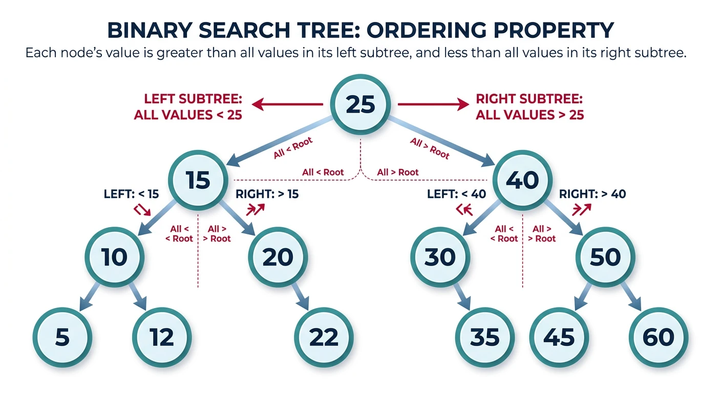
A Binary Search Tree (BST) is a binary tree with an ordering property: for every node, all values in the left subtree are smaller, and all values in the right subtree are larger. This property enables efficient \(O(\log n)\) average-case operations.

Binary search tree with nodes showing left-smaller and right-larger ordering property — Binary Search Tree ordering property: every left subtree contains smaller values and every right subtree contains larger values

BST Property

For every node N: left_subtree_values < N.val < right_subtree_values

This invariant must hold for the entire subtree, not just immediate children!

BST Node Structure

class TreeNode:
    """Binary Search Tree Node"""
    def __init__(self, val=0, left=None, right=None):
        self.val = val
        self.left = left
        self.right = right

class BinarySearchTree:
    """Binary Search Tree implementation"""
    def __init__(self):
        self.root = None
    
    def insert(self, val):
        """Insert a value into the BST"""
        if not self.root:
            self.root = TreeNode(val)
        else:
            self._insert_recursive(self.root, val)
    
    def _insert_recursive(self, node, val):
        """Helper for recursive insertion"""
        if val < node.val:
            if node.left is None:
                node.left = TreeNode(val)
            else:
                self._insert_recursive(node.left, val)
        else:
            if node.right is None:
                node.right = TreeNode(val)
            else:
                self._insert_recursive(node.right, val)
    
    def inorder(self):
        """Return inorder traversal (sorted order)"""
        result = []
        self._inorder_recursive(self.root, result)
        return result
    
    def _inorder_recursive(self, node, result):
        if node:
            self._inorder_recursive(node.left, result)
            result.append(node.val)
            self._inorder_recursive(node.right, result)

# Example usage
bst = BinarySearchTree()
for val in [50, 30, 70, 20, 40, 60, 80]:
    bst.insert(val)

print("Inorder traversal:", bst.inorder())
# Output: [20, 30, 40, 50, 60, 70, 80]

// Binary Search Tree Implementation
#include <iostream>
#include <vector>

struct TreeNode {
    int val;
    TreeNode* left;
    TreeNode* right;
    TreeNode(int x) : val(x), left(nullptr), right(nullptr) {}
};

class BinarySearchTree {
private:
    TreeNode* root;
    
    void insertRecursive(TreeNode* node, int val) {
        if (val < node->val) {
            if (!node->left) node->left = new TreeNode(val);
            else insertRecursive(node->left, val);
        } else {
            if (!node->right) node->right = new TreeNode(val);
            else insertRecursive(node->right, val);
        }
    }
    
    void inorderRecursive(TreeNode* node, std::vector<int>& result) {
        if (node) {
            inorderRecursive(node->left, result);
            result.push_back(node->val);
            inorderRecursive(node->right, result);
        }
    }
    
public:
    BinarySearchTree() : root(nullptr) {}
    
    void insert(int val) {
        if (!root) root = new TreeNode(val);
        else insertRecursive(root, val);
    }
    
    std::vector<int> inorder() {
        std::vector<int> result;
        inorderRecursive(root, result);
        return result;
    }
};

// Usage: BinarySearchTree bst;
// for (int v : {50, 30, 70, 20, 40, 60, 80}) bst.insert(v);

// Binary Search Tree Implementation
import java.util.*;

class TreeNode {
    int val;
    TreeNode left, right;
    TreeNode(int x) { val = x; }
}

class BinarySearchTree {
    private TreeNode root;
    
    public void insert(int val) {
        if (root == null) root = new TreeNode(val);
        else insertRecursive(root, val);
    }
    
    private void insertRecursive(TreeNode node, int val) {
        if (val < node.val) {
            if (node.left == null) node.left = new TreeNode(val);
            else insertRecursive(node.left, val);
        } else {
            if (node.right == null) node.right = new TreeNode(val);
            else insertRecursive(node.right, val);
        }
    }
    
    public List<Integer> inorder() {
        List<Integer> result = new ArrayList<>();
        inorderRecursive(root, result);
        return result;
    }
    
    private void inorderRecursive(TreeNode node, List<Integer> result) {
        if (node != null) {
            inorderRecursive(node.left, result);
            result.add(node.val);
            inorderRecursive(node.right, result);
        }
    }
}

// Usage: BinarySearchTree bst = new BinarySearchTree();
// for (int v : new int[]{50, 30, 70, 20, 40, 60, 80}) bst.insert(v);

BST Operations

Search Operation

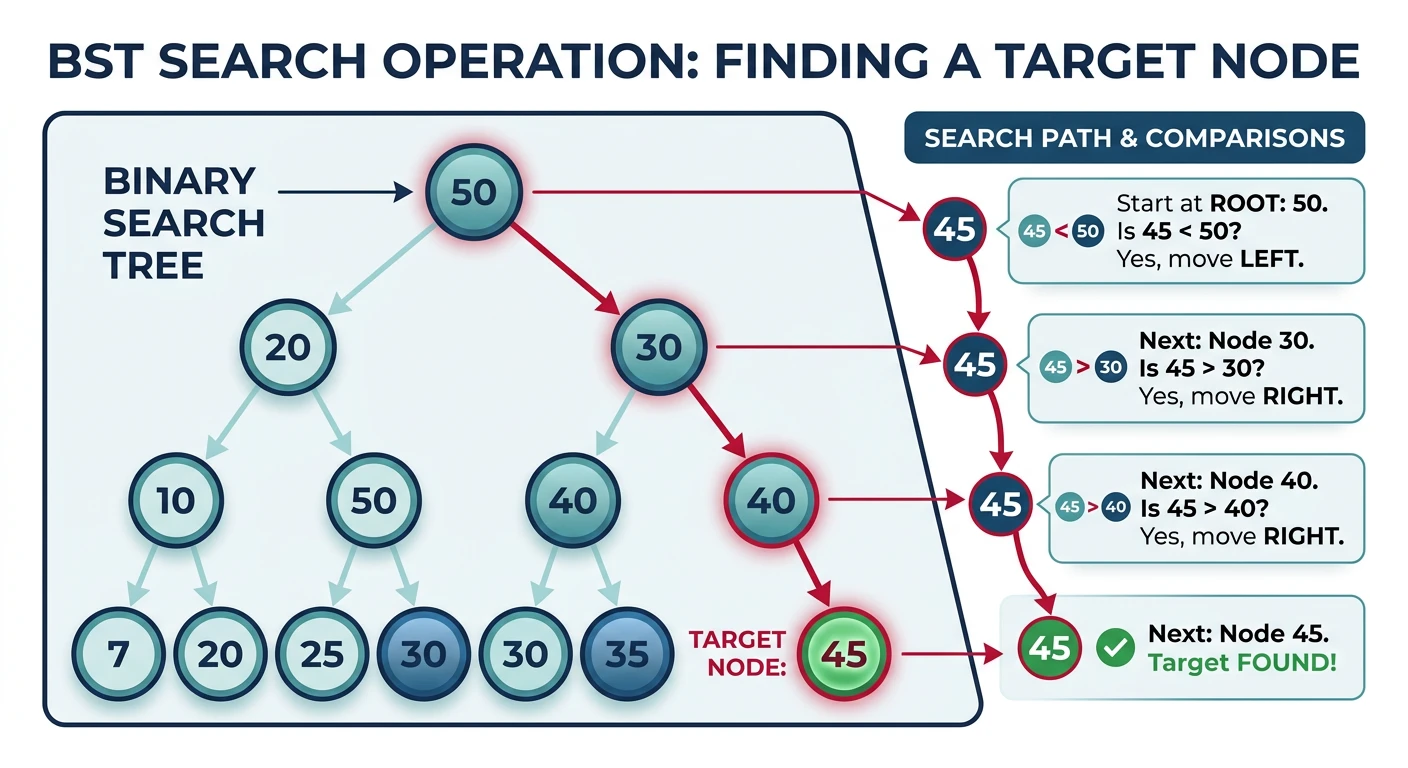
BST search exploits the ordering invariant: at each node, if the target is smaller, go left; if larger, go right. This eliminates half the remaining tree at every step — exactly like binary search on a sorted array, but on a tree structure. Average time: \(O(\log n)\). Worst case (degenerate/skewed tree): \(O(n)\) — which is why balanced variants (AVL, Red-Black) exist.

Iterative vs Recursive: Both work identically. Iterative uses \(O(1)\) space; recursive uses \(O(h)\) call stack space (where \(h\) = tree height). In interviews, iterative is preferred for search since it's simpler and avoids stack overflow on very deep trees.

class TreeNode:
    def __init__(self, val=0, left=None, right=None):
        self.val = val
        self.left = left
        self.right = right

def search_bst(root, target):
    """
    Search for a value in BST
    Time: O(h) where h is height, O(log n) average, O(n) worst
    Space: O(1) iterative
    """
    current = root
    while current:
        if target == current.val:
            return current
        elif target < current.val:
            current = current.left
        else:
            current = current.right
    return None

def search_bst_recursive(root, target):
    """Recursive search implementation"""
    if not root or root.val == target:
        return root
    
    if target < root.val:
        return search_bst_recursive(root.left, target)
    else:
        return search_bst_recursive(root.right, target)

# Build BST: [50, 30, 70, 20, 40, 60, 80]
root = TreeNode(50)
root.left = TreeNode(30)
root.right = TreeNode(70)
root.left.left = TreeNode(20)
root.left.right = TreeNode(40)
root.right.left = TreeNode(60)
root.right.right = TreeNode(80)

# Search for values
result = search_bst(root, 40)
print("Found 40:", result.val if result else "Not found")

result = search_bst(root, 55)
print("Found 55:", result.val if result else "Not found")

// BST Search Operation
// Time: O(h), Space: O(1) iterative
#include <iostream>

struct TreeNode {
    int val;
    TreeNode* left;
    TreeNode* right;
    TreeNode(int x) : val(x), left(nullptr), right(nullptr) {}
};

TreeNode* searchBST(TreeNode* root, int target) {
    TreeNode* current = root;
    while (current) {
        if (target == current->val) return current;
        else if (target < current->val) current = current->left;
        else current = current->right;
    }
    return nullptr;
}

TreeNode* searchBSTRecursive(TreeNode* root, int target) {
    if (!root || root->val == target) return root;
    if (target < root->val) return searchBSTRecursive(root->left, target);
    return searchBSTRecursive(root->right, target);
}

// Usage:
// TreeNode* result = searchBST(root, 40);
// std::cout << (result ? result->val : -1);

// BST Search Operation
// Time: O(h), Space: O(1) iterative

class Solution {
    public TreeNode searchBST(TreeNode root, int target) {
        TreeNode current = root;
        while (current != null) {
            if (target == current.val) return current;
            else if (target < current.val) current = current.left;
            else current = current.right;
        }
        return null;
    }
    
    public TreeNode searchBSTRecursive(TreeNode root, int target) {
        if (root == null || root.val == target) return root;
        if (target < root.val) return searchBSTRecursive(root.left, target);
        return searchBSTRecursive(root.right, target);
    }
}

// Usage:
// TreeNode result = solution.searchBST(root, 40);
// System.out.println(result != null ? result.val : "Not found");

Insert Operation

Insertion follows the same path as search — descend left/right until you find a null position, then attach the new node there. The new node is always inserted as a leaf. This maintains the BST property without rearranging existing nodes (unlike balanced trees which may rotate after insert). Average: \(O(\log n)\). If elements are inserted in sorted order, the tree degenerates to a linked list — \(O(n)\) per operation.

class TreeNode:
    def __init__(self, val=0, left=None, right=None):
        self.val = val
        self.left = left
        self.right = right

def insert_bst(root, val):
    """
    Insert a value into BST
    Time: O(h), Space: O(h) for recursion
    Returns: root of the tree
    """
    if not root:
        return TreeNode(val)
    
    if val < root.val:
        root.left = insert_bst(root.left, val)
    else:
        root.right = insert_bst(root.right, val)
    
    return root

def insert_bst_iterative(root, val):
    """Iterative insertion - O(1) space"""
    new_node = TreeNode(val)
    
    if not root:
        return new_node
    
    current = root
    while True:
        if val < current.val:
            if current.left is None:
                current.left = new_node
                break
            current = current.left
        else:
            if current.right is None:
                current.right = new_node
                break
            current = current.right
    
    return root

# Example: Build BST from scratch
root = None
values = [50, 30, 70, 20, 40, 60, 80, 35]

for val in values:
    root = insert_bst(root, val)

# Verify with inorder traversal
def inorder(node, result=None):
    if result is None:
        result = []
    if node:
        inorder(node.left, result)
        result.append(node.val)
        inorder(node.right, result)
    return result

print("BST inorder:", inorder(root))
# Output: [20, 30, 35, 40, 50, 60, 70, 80]

// BST Insert Operation
// Time: O(h), Space: O(h) recursive, O(1) iterative
#include <iostream>

struct TreeNode {
    int val;
    TreeNode* left;
    TreeNode* right;
    TreeNode(int x) : val(x), left(nullptr), right(nullptr) {}
};

TreeNode* insertBST(TreeNode* root, int val) {
    if (!root) return new TreeNode(val);
    
    if (val < root->val) 
        root->left = insertBST(root->left, val);
    else 
        root->right = insertBST(root->right, val);
    
    return root;
}

TreeNode* insertBSTIterative(TreeNode* root, int val) {
    TreeNode* newNode = new TreeNode(val);
    if (!root) return newNode;
    
    TreeNode* current = root;
    while (true) {
        if (val < current->val) {
            if (!current->left) { current->left = newNode; break; }
            current = current->left;
        } else {
            if (!current->right) { current->right = newNode; break; }
            current = current->right;
        }
    }
    return root;
}

// Usage:
// TreeNode* root = nullptr;
// for (int v : {50, 30, 70, 20, 40}) root = insertBST(root, v);

// BST Insert Operation
// Time: O(h), Space: O(h) recursive, O(1) iterative

class Solution {
    public TreeNode insertBST(TreeNode root, int val) {
        if (root == null) return new TreeNode(val);
        
        if (val < root.val)
            root.left = insertBST(root.left, val);
        else
            root.right = insertBST(root.right, val);
        
        return root;
    }
    
    public TreeNode insertBSTIterative(TreeNode root, int val) {
        TreeNode newNode = new TreeNode(val);
        if (root == null) return newNode;
        
        TreeNode current = root;
        while (true) {
            if (val < current.val) {
                if (current.left == null) { current.left = newNode; break; }
                current = current.left;
            } else {
                if (current.right == null) { current.right = newNode; break; }
                current = current.right;
            }
        }
        return root;
    }
}

// Usage:
// TreeNode root = null;
// for (int v : new int[]{50, 30, 70, 20, 40}) root = solution.insertBST(root, v);

Delete Operation

BST Deletion Cases

Case 1 - Leaf node: Simply remove the node
Case 2 - One child: Replace node with its child
Case 3 - Two children: Replace with inorder successor (or predecessor)

class TreeNode:
    def __init__(self, val=0, left=None, right=None):
        self.val = val
        self.left = left
        self.right = right

def find_min(node):
    """Find minimum value node (leftmost)"""
    current = node
    while current.left:
        current = current.left
    return current

def delete_bst(root, key):
    """
    Delete a node from BST
    Time: O(h), Space: O(h)
    LeetCode 450: Delete Node in a BST
    """
    if not root:
        return None
    
    # Find the node to delete
    if key < root.val:
        root.left = delete_bst(root.left, key)
    elif key > root.val:
        root.right = delete_bst(root.right, key)
    else:
        # Found the node to delete
        
        # Case 1 & 2: Node has 0 or 1 child
        if not root.left:
            return root.right
        elif not root.right:
            return root.left
        
        # Case 3: Node has two children
        # Find inorder successor (smallest in right subtree)
        successor = find_min(root.right)
        
        # Copy successor's value to this node
        root.val = successor.val
        
        # Delete the successor
        root.right = delete_bst(root.right, successor.val)
    
    return root

# Build BST
def build_bst(values):
    root = None
    for val in values:
        if not root:
            root = TreeNode(val)
        else:
            curr = root
            while True:
                if val < curr.val:
                    if not curr.left:
                        curr.left = TreeNode(val)
                        break
                    curr = curr.left
                else:
                    if not curr.right:
                        curr.right = TreeNode(val)
                        break
                    curr = curr.right
    return root

def inorder(node):
    if not node:
        return []
    return inorder(node.left) + [node.val] + inorder(node.right)

root = build_bst([50, 30, 70, 20, 40, 60, 80])
print("Before delete:", inorder(root))

root = delete_bst(root, 30)  # Delete node with two children
print("After delete 30:", inorder(root))

root = delete_bst(root, 20)  # Delete leaf
print("After delete 20:", inorder(root))

// BST Delete Operation - LeetCode 450
// Time: O(h), Space: O(h)
#include <iostream>

struct TreeNode {
    int val;
    TreeNode* left;
    TreeNode* right;
    TreeNode(int x) : val(x), left(nullptr), right(nullptr) {}
};

TreeNode* findMin(TreeNode* node) {
    while (node->left) node = node->left;
    return node;
}

TreeNode* deleteBST(TreeNode* root, int key) {
    if (!root) return nullptr;
    
    if (key < root->val) {
        root->left = deleteBST(root->left, key);
    } else if (key > root->val) {
        root->right = deleteBST(root->right, key);
    } else {
        // Case 1 & 2: Node has 0 or 1 child
        if (!root->left) return root->right;
        if (!root->right) return root->left;
        
        // Case 3: Two children - find inorder successor
        TreeNode* successor = findMin(root->right);
        root->val = successor->val;
        root->right = deleteBST(root->right, successor->val);
    }
    return root;
}

// Usage:
// root = deleteBST(root, 30);  // Delete node with two children

// BST Delete Operation - LeetCode 450
// Time: O(h), Space: O(h)

class Solution {
    private TreeNode findMin(TreeNode node) {
        while (node.left != null) node = node.left;
        return node;
    }
    
    public TreeNode deleteNode(TreeNode root, int key) {
        if (root == null) return null;
        
        if (key < root.val) {
            root.left = deleteNode(root.left, key);
        } else if (key > root.val) {
            root.right = deleteNode(root.right, key);
        } else {
            // Case 1 & 2: Node has 0 or 1 child
            if (root.left == null) return root.right;
            if (root.right == null) return root.left;
            
            // Case 3: Two children - find inorder successor
            TreeNode successor = findMin(root.right);
            root.val = successor.val;
            root.right = deleteNode(root.right, successor.val);
        }
        return root;
    }
}

// Usage:
// root = solution.deleteNode(root, 30);  // Delete node with two children

Inorder Successor & Predecessor

The inorder successor of a node is the next node in sorted order — the smallest value greater than the current node. Two cases: (1) If the node has a right subtree, the successor is the leftmost node in the right subtree. (2) If no right subtree, walk up to the first ancestor where the node is in its left subtree. This concept is critical for BST deletion (Case 3) and for building iterators over BSTs.

class TreeNode:
    def __init__(self, val=0, left=None, right=None):
        self.val = val
        self.left = left
        self.right = right

def inorder_successor(root, target):
    """
    Find inorder successor of a node with given value
    Time: O(h), Space: O(1)
    """
    successor = None
    current = root
    
    while current:
        if target < current.val:
            successor = current  # Potential successor
            current = current.left
        else:
            current = current.right
    
    return successor

def inorder_predecessor(root, target):
    """
    Find inorder predecessor of a node with given value
    Time: O(h), Space: O(1)
    """
    predecessor = None
    current = root
    
    while current:
        if target > current.val:
            predecessor = current  # Potential predecessor
            current = current.right
        else:
            current = current.left
    
    return predecessor

# Build BST: [20, 30, 40, 50, 60, 70, 80]
root = TreeNode(50)
root.left = TreeNode(30, TreeNode(20), TreeNode(40))
root.right = TreeNode(70, TreeNode(60), TreeNode(80))

# Find successor of 40 (should be 50)
succ = inorder_successor(root, 40)
print(f"Successor of 40: {succ.val if succ else None}")

# Find predecessor of 60 (should be 50)
pred = inorder_predecessor(root, 60)
print(f"Predecessor of 60: {pred.val if pred else None}")

# Find successor of 80 (should be None)
succ = inorder_successor(root, 80)
print(f"Successor of 80: {succ.val if succ else None}")

// Inorder Successor and Predecessor in BST
// Time: O(h), Space: O(1)
#include <iostream>

struct TreeNode {
    int val;
    TreeNode* left;
    TreeNode* right;
    TreeNode(int x) : val(x), left(nullptr), right(nullptr) {}
};

TreeNode* inorderSuccessor(TreeNode* root, int target) {
    TreeNode* successor = nullptr;
    TreeNode* current = root;
    
    while (current) {
        if (target < current->val) {
            successor = current;  // Potential successor
            current = current->left;
        } else {
            current = current->right;
        }
    }
    return successor;
}

TreeNode* inorderPredecessor(TreeNode* root, int target) {
    TreeNode* predecessor = nullptr;
    TreeNode* current = root;
    
    while (current) {
        if (target > current->val) {
            predecessor = current;  // Potential predecessor
            current = current->right;
        } else {
            current = current->left;
        }
    }
    return predecessor;
}

// Usage:
// TreeNode* succ = inorderSuccessor(root, 40);  // Returns node with value 50
// TreeNode* pred = inorderPredecessor(root, 60); // Returns node with value 50

// Inorder Successor and Predecessor in BST
// Time: O(h), Space: O(1)

class Solution {
    public TreeNode inorderSuccessor(TreeNode root, int target) {
        TreeNode successor = null;
        TreeNode current = root;
        
        while (current != null) {
            if (target < current.val) {
                successor = current;  // Potential successor
                current = current.left;
            } else {
                current = current.right;
            }
        }
        return successor;
    }
    
    public TreeNode inorderPredecessor(TreeNode root, int target) {
        TreeNode predecessor = null;
        TreeNode current = root;
        
        while (current != null) {
            if (target > current.val) {
                predecessor = current;  // Potential predecessor
                current = current.right;
            } else {
                current = current.left;
            }
        }
        return predecessor;
    }
}

// Usage:
// TreeNode succ = solution.inorderSuccessor(root, 40);  // Returns node with value 50
// TreeNode pred = solution.inorderPredecessor(root, 60); // Returns node with value 50

BST Validation

class TreeNode:
    def __init__(self, val=0, left=None, right=None):
        self.val = val
        self.left = left
        self.right = right

def is_valid_bst(root):
    """
    Validate Binary Search Tree
    LeetCode 98: Validate Binary Search Tree
    Time: O(n), Space: O(h)
    """
    def validate(node, min_val, max_val):
        if not node:
            return True
        
        # Check current node's value against bounds
        if node.val <= min_val or node.val >= max_val:
            return False
        
        # Recursively validate left and right subtrees
        # Left subtree: all values must be < current node's value
        # Right subtree: all values must be > current node's value
        return (validate(node.left, min_val, node.val) and
                validate(node.right, node.val, max_val))
    
    return validate(root, float('-inf'), float('inf'))

def is_valid_bst_inorder(root):
    """
    Validate BST using inorder traversal
    Inorder of BST should be strictly increasing
    """
    prev = float('-inf')
    
    def inorder(node):
        nonlocal prev
        if not node:
            return True
        
        # Check left subtree
        if not inorder(node.left):
            return False
        
        # Check current node
        if node.val <= prev:
            return False
        prev = node.val
        
        # Check right subtree
        return inorder(node.right)
    
    return inorder(root)

# Test cases
# Valid BST
valid_root = TreeNode(5, TreeNode(3, TreeNode(1), TreeNode(4)),
                         TreeNode(7, TreeNode(6), TreeNode(8)))
print("Valid BST:", is_valid_bst(valid_root))  # True

# Invalid BST (4 is in right subtree but < 5)
invalid_root = TreeNode(5, TreeNode(1), TreeNode(4, TreeNode(3), TreeNode(6)))
print("Invalid BST:", is_valid_bst(invalid_root))  # False

// LeetCode 98 - Validate Binary Search Tree
// Time: O(n), Space: O(h)
#include <climits>

struct TreeNode {
    int val;
    TreeNode* left;
    TreeNode* right;
    TreeNode(int x) : val(x), left(nullptr), right(nullptr) {}
};

class Solution {
private:
    bool validate(TreeNode* node, long minVal, long maxVal) {
        if (!node) return true;
        
        if (node->val <= minVal || node->val >= maxVal)
            return false;
        
        return validate(node->left, minVal, node->val) &&
               validate(node->right, node->val, maxVal);
    }
    
public:
    bool isValidBST(TreeNode* root) {
        return validate(root, LONG_MIN, LONG_MAX);
    }
    
    // Alternative: Inorder traversal approach
    bool isValidBSTInorder(TreeNode* root) {
        long prev = LONG_MIN;
        return inorder(root, prev);
    }
    
    bool inorder(TreeNode* node, long& prev) {
        if (!node) return true;
        if (!inorder(node->left, prev)) return false;
        if (node->val <= prev) return false;
        prev = node->val;
        return inorder(node->right, prev);
    }
};

// LeetCode 98 - Validate Binary Search Tree
// Time: O(n), Space: O(h)

class Solution {
    public boolean isValidBST(TreeNode root) {
        return validate(root, Long.MIN_VALUE, Long.MAX_VALUE);
    }
    
    private boolean validate(TreeNode node, long minVal, long maxVal) {
        if (node == null) return true;
        
        if (node.val <= minVal || node.val >= maxVal)
            return false;
        
        return validate(node.left, minVal, node.val) &&
               validate(node.right, node.val, maxVal);
    }
    
    // Alternative: Inorder traversal approach
    private long prev = Long.MIN_VALUE;
    
    public boolean isValidBSTInorder(TreeNode root) {
        prev = Long.MIN_VALUE;
        return inorder(root);
    }
    
    private boolean inorder(TreeNode node) {
        if (node == null) return true;
        if (!inorder(node.left)) return false;
        if (node.val <= prev) return false;
        prev = node.val;
        return inorder(node.right);
    }
}

AVL Trees

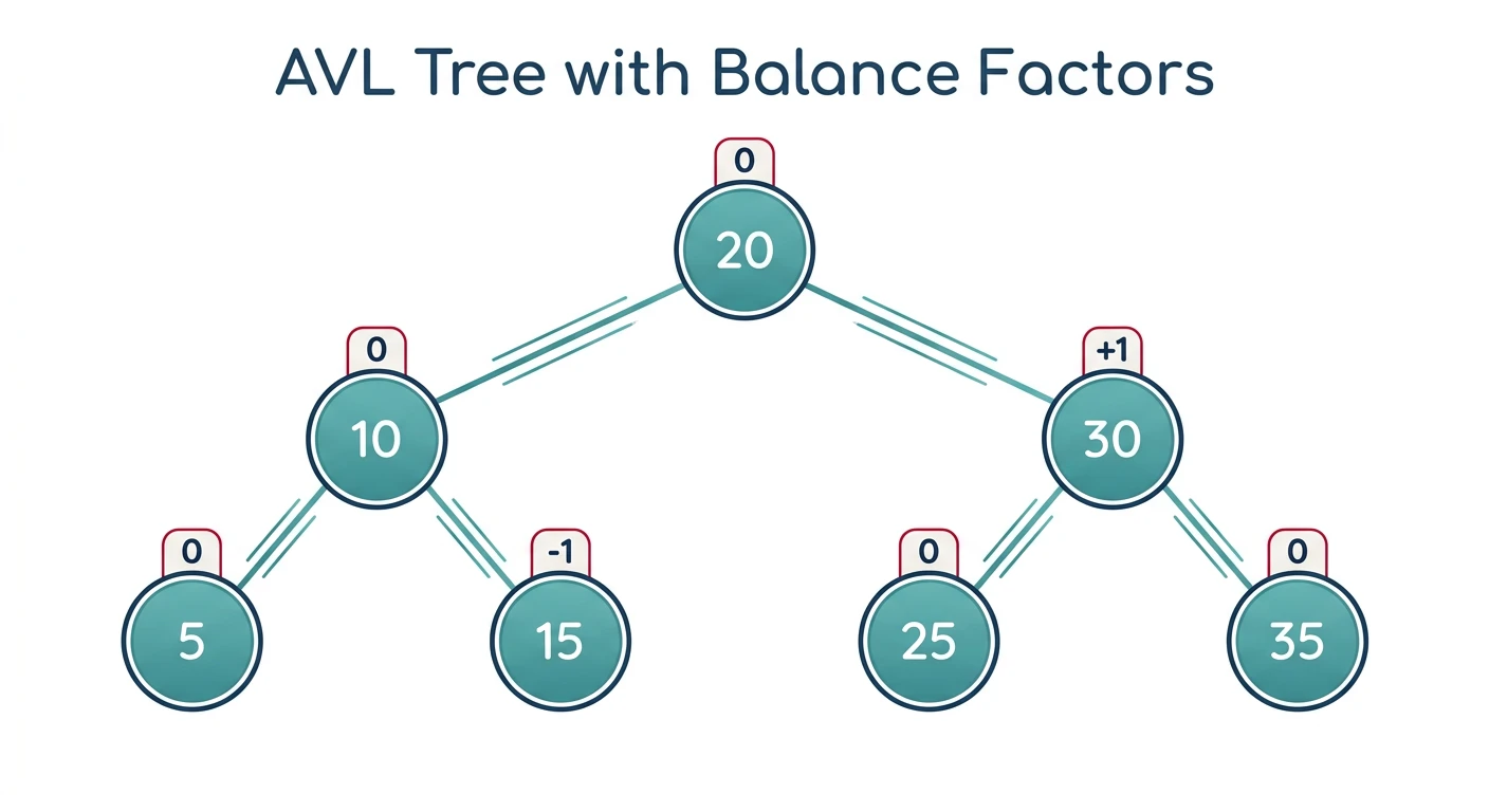
AVL Tree is a self-balancing BST where the height difference between left and right subtrees (balance factor) is at most 1 for every node. Named after inventors Adelson-Velsky and Landis.

AVL tree with balance factors labeled at each node showing -1, 0, and +1 values — AVL tree with balance factors: each node maintains |balance factor| ≤ 1, ensuring \(O(\log n)\) height guarantee

AVL Property

Balance Factor = height(left subtree) - height(right subtree)

Valid balance factors: -1, 0, +1

If |balance factor| > 1, tree needs rebalancing via rotations.

AVL Node Structure

class AVLNode:
    """AVL Tree Node with height tracking"""
    def __init__(self, val):
        self.val = val
        self.left = None
        self.right = None
        self.height = 1  # Height of node (leaf = 1)

class AVLTree:
    """AVL Tree implementation"""
    
    def __init__(self):
        self.root = None
    
    def get_height(self, node):
        """Get height of node (None has height 0)"""
        if not node:
            return 0
        return node.height
    
    def get_balance(self, node):
        """Get balance factor of node"""
        if not node:
            return 0
        return self.get_height(node.left) - self.get_height(node.right)
    
    def update_height(self, node):
        """Update height of node based on children"""
        if node:
            node.height = 1 + max(self.get_height(node.left),
                                   self.get_height(node.right))
    
    def inorder(self):
        """Return inorder traversal"""
        result = []
        self._inorder(self.root, result)
        return result
    
    def _inorder(self, node, result):
        if node:
            self._inorder(node.left, result)
            result.append(node.val)
            self._inorder(node.right, result)

# Example
tree = AVLTree()
root = AVLNode(10)
root.left = AVLNode(5)
root.right = AVLNode(15)
root.left.left = AVLNode(2)

tree.root = root
tree.update_height(root.left)
tree.update_height(root)

print(f"Root height: {root.height}")
print(f"Root balance: {tree.get_balance(root)}")
print(f"Left child balance: {tree.get_balance(root.left)}")

// AVL Tree Node Structure
#include <iostream>
#include <algorithm>

struct AVLNode {
    int val;
    AVLNode* left;
    AVLNode* right;
    int height;
    AVLNode(int x) : val(x), left(nullptr), right(nullptr), height(1) {}
};

class AVLTree {
private:
    AVLNode* root;
    
    int getHeight(AVLNode* node) {
        return node ? node->height : 0;
    }
    
    int getBalance(AVLNode* node) {
        return node ? getHeight(node->left) - getHeight(node->right) : 0;
    }
    
    void updateHeight(AVLNode* node) {
        if (node) {
            node->height = 1 + std::max(getHeight(node->left), 
                                         getHeight(node->right));
        }
    }
    
public:
    AVLTree() : root(nullptr) {}
    
    void printInfo(AVLNode* node) {
        if (node) {
            std::cout << "Value: " << node->val 
                      << ", Height: " << node->height
                      << ", Balance: " << getBalance(node) << std::endl;
        }
    }
};

// AVL Tree Node Structure

class AVLNode {
    int val;
    AVLNode left, right;
    int height;
    
    AVLNode(int x) {
        val = x;
        height = 1;
    }
}

class AVLTree {
    private AVLNode root;
    
    private int getHeight(AVLNode node) {
        return node != null ? node.height : 0;
    }
    
    private int getBalance(AVLNode node) {
        return node != null ? getHeight(node.left) - getHeight(node.right) : 0;
    }
    
    private void updateHeight(AVLNode node) {
        if (node != null) {
            node.height = 1 + Math.max(getHeight(node.left), 
                                        getHeight(node.right));
        }
    }
    
    public void printInfo(AVLNode node) {
        if (node != null) {
            System.out.println("Value: " + node.val + 
                             ", Height: " + node.height +
                             ", Balance: " + getBalance(node));
        }
    }
}

AVL Rotations

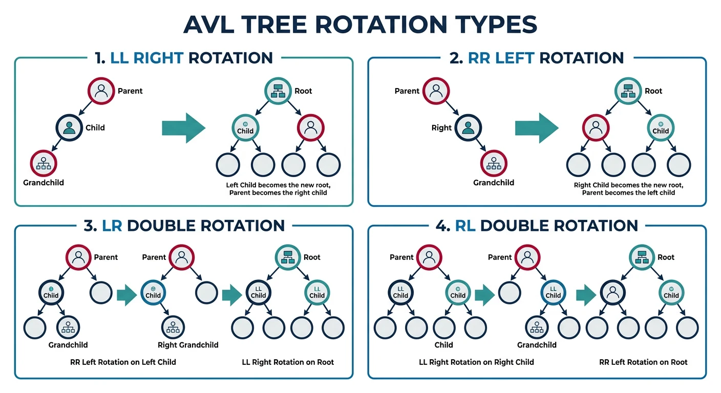
Four Types of Rotations

Imbalance	Rotation	When to Use
Left-Left (LL)	Right Rotation	balance > 1 AND left balance >= 0
Right-Right (RR)	Left Rotation	balance < -1 AND right balance <= 0
Left-Right (LR)	Left then Right	balance > 1 AND left balance < 0
Right-Left (RL)	Right then Left	balance < -1 AND right balance > 0

Four AVL rotation types: LL right rotation, RR left rotation, LR double rotation, RL double rotation — Four AVL rotation types: LL (right rotation), RR (left rotation), LR (left-right double rotation), and RL (right-left double rotation)

AVL Rebalancing Decision Flow

                            flowchart TD
                                A["Insert/Delete Node"] --> B{"Update Heights"}
                                B --> C{"Balance Factor?"}
                                C -->|"BF > 1
(Left Heavy)"| D{"Left Child BF?"}
                                C -->|"-1 ≤ BF ≤ 1
(Balanced)"| E["No Rotation Needed"]
                                C -->|"BF < -1
(Right Heavy)"| F{"Right Child BF?"}
                                D -->|"≥ 0 (LL Case)"| G["Right Rotate"]
                                D -->|"< 0 (LR Case)"| H["Left Rotate Child →
Right Rotate Node"]
                                F -->|"≤ 0 (RR Case)"| I["Left Rotate"]
                                F -->|"> 0 (RL Case)"| J["Right Rotate Child →
Left Rotate Node"]
                                G --> K["Tree Balanced ✓"]
                                H --> K
                                I --> K
                                J --> K

Interactive: AVL Left Rotation (RR Case)

Step through a left rotation to see how an unbalanced RR case is resolved. Use the Next button to advance each stage.

AVL Left Rotation — Step-Through

Unbalanced Rotating Balanced Subtree

Unbalanced Tree (RR Case)

After inserting node X, Z has balance factor -2. Click Next to walk through the left rotation.

Before rotation Step 1 / 4

class AVLNode:
    def __init__(self, val):
        self.val = val
        self.left = None
        self.right = None
        self.height = 1

class AVLTree:
    def get_height(self, node):
        return node.height if node else 0
    
    def get_balance(self, node):
        return self.get_height(node.left) - self.get_height(node.right) if node else 0
    
    def update_height(self, node):
        if node:
            node.height = 1 + max(self.get_height(node.left),
                                   self.get_height(node.right))
    
    def right_rotate(self, y):
        """
        Right rotation (LL case)
        
             y                x
            / \             /   \
           x   T3   -->    T1    y
          / \                   / \
         T1  T2               T2  T3
        """
        x = y.left
        T2 = x.right
        
        # Perform rotation
        x.right = y
        y.left = T2
        
        # Update heights (y first, then x)
        self.update_height(y)
        self.update_height(x)
        
        return x  # New root
    
    def left_rotate(self, x):
        """
        Left rotation (RR case)
        
           x                    y
          / \                 /   \
         T1  y      -->      x    T3
            / \             / \
           T2  T3          T1  T2
        """
        y = x.right
        T2 = y.left
        
        # Perform rotation
        y.left = x
        x.right = T2
        
        # Update heights (x first, then y)
        self.update_height(x)
        self.update_height(y)
        
        return y  # New root
    
    def insert(self, root, val):
        """Insert value and rebalance"""
        # Step 1: Normal BST insertion
        if not root:
            return AVLNode(val)
        
        if val < root.val:
            root.left = self.insert(root.left, val)
        else:
            root.right = self.insert(root.right, val)
        
        # Step 2: Update height
        self.update_height(root)
        
        # Step 3: Get balance factor
        balance = self.get_balance(root)
        
        # Step 4: Rebalance if needed
        
        # Left Left Case (LL)
        if balance > 1 and val < root.left.val:
            return self.right_rotate(root)
        
        # Right Right Case (RR)
        if balance < -1 and val > root.right.val:
            return self.left_rotate(root)
        
        # Left Right Case (LR)
        if balance > 1 and val > root.left.val:
            root.left = self.left_rotate(root.left)
            return self.right_rotate(root)
        
        # Right Left Case (RL)
        if balance < -1 and val < root.right.val:
            root.right = self.right_rotate(root.right)
            return self.left_rotate(root)
        
        return root

# Example: Insert values and observe balancing
avl = AVLTree()
root = None

values = [10, 20, 30, 40, 50, 25]
for val in values:
    root = avl.insert(root, val)
    print(f"Inserted {val}, root = {root.val}, balance = {avl.get_balance(root)}")

def inorder(node):
    return inorder(node.left) + [node.val] + inorder(node.right) if node else []

print("Inorder:", inorder(root))

// AVL Tree with Rotations
#include <iostream>
#include <algorithm>

struct AVLNode {
    int val, height;
    AVLNode *left, *right;
    AVLNode(int x) : val(x), height(1), left(nullptr), right(nullptr) {}
};

class AVLTree {
private:
    int getHeight(AVLNode* n) { return n ? n->height : 0; }
    int getBalance(AVLNode* n) { return n ? getHeight(n->left) - getHeight(n->right) : 0; }
    void updateHeight(AVLNode* n) { 
        if (n) n->height = 1 + std::max(getHeight(n->left), getHeight(n->right)); 
    }
    
    AVLNode* rightRotate(AVLNode* y) {
        AVLNode* x = y->left;
        y->left = x->right;
        x->right = y;
        updateHeight(y); updateHeight(x);
        return x;
    }
    
    AVLNode* leftRotate(AVLNode* x) {
        AVLNode* y = x->right;
        x->right = y->left;
        y->left = x;
        updateHeight(x); updateHeight(y);
        return y;
    }
    
public:
    AVLNode* insert(AVLNode* root, int val) {
        if (!root) return new AVLNode(val);
        if (val < root->val) root->left = insert(root->left, val);
        else root->right = insert(root->right, val);
        
        updateHeight(root);
        int bal = getBalance(root);
        
        if (bal > 1 && val < root->left->val) return rightRotate(root);  // LL
        if (bal < -1 && val > root->right->val) return leftRotate(root);  // RR
        if (bal > 1 && val > root->left->val) {                           // LR
            root->left = leftRotate(root->left);
            return rightRotate(root);
        }
        if (bal < -1 && val < root->right->val) {                         // RL
            root->right = rightRotate(root->right);
            return leftRotate(root);
        }
        return root;
    }
};

// AVL Tree with Rotations

class AVLNode {
    int val, height;
    AVLNode left, right;
    AVLNode(int x) { val = x; height = 1; }
}

class AVLTree {
    private int getHeight(AVLNode n) { return n != null ? n.height : 0; }
    private int getBalance(AVLNode n) { 
        return n != null ? getHeight(n.left) - getHeight(n.right) : 0; 
    }
    private void updateHeight(AVLNode n) { 
        if (n != null) n.height = 1 + Math.max(getHeight(n.left), getHeight(n.right)); 
    }
    
    private AVLNode rightRotate(AVLNode y) {
        AVLNode x = y.left;
        y.left = x.right;
        x.right = y;
        updateHeight(y); updateHeight(x);
        return x;
    }
    
    private AVLNode leftRotate(AVLNode x) {
        AVLNode y = x.right;
        x.right = y.left;
        y.left = x;
        updateHeight(x); updateHeight(y);
        return y;
    }
    
    public AVLNode insert(AVLNode root, int val) {
        if (root == null) return new AVLNode(val);
        if (val < root.val) root.left = insert(root.left, val);
        else root.right = insert(root.right, val);
        
        updateHeight(root);
        int bal = getBalance(root);
        
        if (bal > 1 && val < root.left.val) return rightRotate(root);  // LL
        if (bal < -1 && val > root.right.val) return leftRotate(root); // RR
        if (bal > 1 && val > root.left.val) {                          // LR
            root.left = leftRotate(root.left);
            return rightRotate(root);
        }
        if (bal < -1 && val < root.right.val) {                        // RL
            root.right = rightRotate(root.right);
            return leftRotate(root);
        }
        return root;
    }
}

Complete AVL Insert with All Cases

class AVLNode:
    def __init__(self, val):
        self.val = val
        self.left = None
        self.right = None
        self.height = 1

class AVLTree:
    def __init__(self):
        self.root = None
    
    def height(self, node):
        return node.height if node else 0
    
    def balance(self, node):
        return self.height(node.left) - self.height(node.right) if node else 0
    
    def right_rotate(self, y):
        x = y.left
        T2 = x.right
        x.right = y
        y.left = T2
        y.height = 1 + max(self.height(y.left), self.height(y.right))
        x.height = 1 + max(self.height(x.left), self.height(x.right))
        return x
    
    def left_rotate(self, x):
        y = x.right
        T2 = y.left
        y.left = x
        x.right = T2
        x.height = 1 + max(self.height(x.left), self.height(x.right))
        y.height = 1 + max(self.height(y.left), self.height(y.right))
        return y
    
    def insert(self, val):
        self.root = self._insert(self.root, val)
    
    def _insert(self, node, val):
        # BST insert
        if not node:
            return AVLNode(val)
        if val < node.val:
            node.left = self._insert(node.left, val)
        else:
            node.right = self._insert(node.right, val)
        
        # Update height
        node.height = 1 + max(self.height(node.left), self.height(node.right))
        
        # Get balance
        bal = self.balance(node)
        
        # LL Case
        if bal > 1 and val < node.left.val:
            return self.right_rotate(node)
        
        # RR Case
        if bal < -1 and val > node.right.val:
            return self.left_rotate(node)
        
        # LR Case
        if bal > 1 and val > node.left.val:
            node.left = self.left_rotate(node.left)
            return self.right_rotate(node)
        
        # RL Case
        if bal < -1 and val < node.right.val:
            node.right = self.right_rotate(node.right)
            return self.left_rotate(node)
        
        return node
    
    def delete(self, val):
        self.root = self._delete(self.root, val)
    
    def _delete(self, node, val):
        if not node:
            return node
        
        # BST delete
        if val < node.val:
            node.left = self._delete(node.left, val)
        elif val > node.val:
            node.right = self._delete(node.right, val)
        else:
            # Node to delete found
            if not node.left:
                return node.right
            elif not node.right:
                return node.left
            
            # Two children: get inorder successor
            temp = self._min_node(node.right)
            node.val = temp.val
            node.right = self._delete(node.right, temp.val)
        
        if not node:
            return node
        
        # Update height
        node.height = 1 + max(self.height(node.left), self.height(node.right))
        
        # Rebalance
        bal = self.balance(node)
        
        # LL
        if bal > 1 and self.balance(node.left) >= 0:
            return self.right_rotate(node)
        
        # LR
        if bal > 1 and self.balance(node.left) < 0:
            node.left = self.left_rotate(node.left)
            return self.right_rotate(node)
        
        # RR
        if bal < -1 and self.balance(node.right) <= 0:
            return self.left_rotate(node)
        
        # RL
        if bal < -1 and self.balance(node.right) > 0:
            node.right = self.right_rotate(node.right)
            return self.left_rotate(node)
        
        return node
    
    def _min_node(self, node):
        while node.left:
            node = node.left
        return node
    
    def levelorder(self):
        if not self.root:
            return []
        from collections import deque
        result = []
        queue = deque([self.root])
        while queue:
            node = queue.popleft()
            result.append(f"{node.val}(h={node.height})")
            if node.left:
                queue.append(node.left)
            if node.right:
                queue.append(node.right)
        return result

# Example usage
avl = AVLTree()
for val in [10, 20, 30, 15, 25, 5, 1]:
    avl.insert(val)
    print(f"After insert {val}: {avl.levelorder()}")

print("\nDeleting 20...")
avl.delete(20)
print(f"After delete: {avl.levelorder()}")

// Complete AVL Tree with Insert and Delete
#include <iostream>
#include <algorithm>
#include <queue>
#include <string>

struct AVLNode {
    int val, height;
    AVLNode *left, *right;
    AVLNode(int x) : val(x), height(1), left(nullptr), right(nullptr) {}
};

class AVLTree {
private:
    AVLNode* root = nullptr;
    int h(AVLNode* n) { return n ? n->height : 0; }
    int bal(AVLNode* n) { return n ? h(n->left) - h(n->right) : 0; }
    void upd(AVLNode* n) { if (n) n->height = 1 + std::max(h(n->left), h(n->right)); }
    
    AVLNode* rr(AVLNode* y) { AVLNode* x = y->left; y->left = x->right; x->right = y; upd(y); upd(x); return x; }
    AVLNode* lr(AVLNode* x) { AVLNode* y = x->right; x->right = y->left; y->left = x; upd(x); upd(y); return y; }
    AVLNode* minNode(AVLNode* n) { while (n->left) n = n->left; return n; }
    
    AVLNode* rebalance(AVLNode* n, int val, bool isInsert) {
        upd(n); int b = bal(n);
        if (isInsert) {
            if (b > 1 && val < n->left->val) return rr(n);
            if (b < -1 && val > n->right->val) return lr(n);
            if (b > 1 && val > n->left->val) { n->left = lr(n->left); return rr(n); }
            if (b < -1 && val < n->right->val) { n->right = rr(n->right); return lr(n); }
        } else {
            if (b > 1 && bal(n->left) >= 0) return rr(n);
            if (b > 1 && bal(n->left) < 0) { n->left = lr(n->left); return rr(n); }
            if (b < -1 && bal(n->right) <= 0) return lr(n);
            if (b < -1 && bal(n->right) > 0) { n->right = rr(n->right); return lr(n); }
        }
        return n;
    }
    
    AVLNode* ins(AVLNode* n, int val) {
        if (!n) return new AVLNode(val);
        if (val < n->val) n->left = ins(n->left, val);
        else n->right = ins(n->right, val);
        return rebalance(n, val, true);
    }
    
    AVLNode* del(AVLNode* n, int val) {
        if (!n) return n;
        if (val < n->val) n->left = del(n->left, val);
        else if (val > n->val) n->right = del(n->right, val);
        else {
            if (!n->left) return n->right;
            if (!n->right) return n->left;
            AVLNode* temp = minNode(n->right);
            n->val = temp->val;
            n->right = del(n->right, temp->val);
        }
        return rebalance(n, val, false);
    }
    
public:
    void insert(int val) { root = ins(root, val); }
    void remove(int val) { root = del(root, val); }
};

// Complete AVL Tree with Insert and Delete
import java.util.*;

class AVLNode {
    int val, height;
    AVLNode left, right;
    AVLNode(int x) { val = x; height = 1; }
}

class AVLTree {
    private AVLNode root;
    private int h(AVLNode n) { return n != null ? n.height : 0; }
    private int bal(AVLNode n) { return n != null ? h(n.left) - h(n.right) : 0; }
    private void upd(AVLNode n) { if (n != null) n.height = 1 + Math.max(h(n.left), h(n.right)); }
    
    private AVLNode rr(AVLNode y) { 
        AVLNode x = y.left; y.left = x.right; x.right = y; upd(y); upd(x); return x; 
    }
    private AVLNode lr(AVLNode x) { 
        AVLNode y = x.right; x.right = y.left; y.left = x; upd(x); upd(y); return y; 
    }
    private AVLNode minNode(AVLNode n) { while (n.left != null) n = n.left; return n; }
    
    private AVLNode rebalance(AVLNode n, int val, boolean isInsert) {
        upd(n); int b = bal(n);
        if (isInsert) {
            if (b > 1 && val < n.left.val) return rr(n);
            if (b < -1 && val > n.right.val) return lr(n);
            if (b > 1 && val > n.left.val) { n.left = lr(n.left); return rr(n); }
            if (b < -1 && val < n.right.val) { n.right = rr(n.right); return lr(n); }
        } else {
            if (b > 1 && bal(n.left) >= 0) return rr(n);
            if (b > 1 && bal(n.left) < 0) { n.left = lr(n.left); return rr(n); }
            if (b < -1 && bal(n.right) <= 0) return lr(n);
            if (b < -1 && bal(n.right) > 0) { n.right = rr(n.right); return lr(n); }
        }
        return n;
    }
    
    private AVLNode ins(AVLNode n, int val) {
        if (n == null) return new AVLNode(val);
        if (val < n.val) n.left = ins(n.left, val);
        else n.right = ins(n.right, val);
        return rebalance(n, val, true);
    }
    
    private AVLNode del(AVLNode n, int val) {
        if (n == null) return n;
        if (val < n.val) n.left = del(n.left, val);
        else if (val > n.val) n.right = del(n.right, val);
        else {
            if (n.left == null) return n.right;
            if (n.right == null) return n.left;
            AVLNode temp = minNode(n.right);
            n.val = temp.val;
            n.right = del(n.right, temp.val);
        }
        return rebalance(n, val, false);
    }
    
    public void insert(int val) { root = ins(root, val); }
    public void remove(int val) { root = del(root, val); }
}

Red-Black Trees

Red-Black Tree is another self-balancing BST with less strict balancing than AVL. It uses node coloring to maintain approximate balance, guaranteeing \(O(\log n)\) operations.

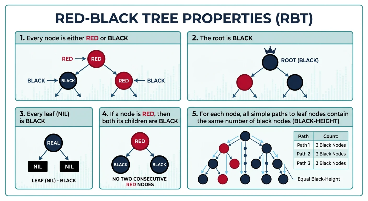
Red-Black tree with nodes colored red and black showing all five properties satisfied — Red-Black tree: nodes colored red or black satisfying five properties including black-height consistency and no consecutive red nodes

                            Red-Black Properties
                            Every node is either RED or BLACK
Root is always BLACK
All leaves (NIL nodes) are BLACK
Red node cannot have red children (no two reds in a row)
Every path from root to leaf has same number of black nodes (black height)

                        

class Color:
    RED = True
    BLACK = False

class RBNode:
    """Red-Black Tree Node"""
    def __init__(self, val, color=Color.RED):
        self.val = val
        self.color = color
        self.left = None
        self.right = None
        self.parent = None

class RedBlackTree:
    """
    Red-Black Tree implementation
    Note: Simplified version for understanding concepts
    """
    def __init__(self):
        self.NIL = RBNode(None, Color.BLACK)  # Sentinel nil node
        self.root = self.NIL
    
    def left_rotate(self, x):
        """Left rotation around x"""
        y = x.right
        x.right = y.left
        
        if y.left != self.NIL:
            y.left.parent = x
        
        y.parent = x.parent
        
        if x.parent is None:
            self.root = y
        elif x == x.parent.left:
            x.parent.left = y
        else:
            x.parent.right = y
        
        y.left = x
        x.parent = y
    
    def right_rotate(self, y):
        """Right rotation around y"""
        x = y.left
        y.left = x.right
        
        if x.right != self.NIL:
            x.right.parent = y
        
        x.parent = y.parent
        
        if y.parent is None:
            self.root = x
        elif y == y.parent.right:
            y.parent.right = x
        else:
            y.parent.left = x
        
        x.right = y
        y.parent = x
    
    def insert(self, val):
        """Insert value into Red-Black Tree"""
        new_node = RBNode(val)
        new_node.left = self.NIL
        new_node.right = self.NIL
        
        # BST insert
        parent = None
        current = self.root
        
        while current != self.NIL:
            parent = current
            if val < current.val:
                current = current.left
            else:
                current = current.right
        
        new_node.parent = parent
        
        if parent is None:
            self.root = new_node
        elif val < parent.val:
            parent.left = new_node
        else:
            parent.right = new_node
        
        # Fix Red-Black properties
        self._fix_insert(new_node)
    
    def _fix_insert(self, k):
        """Fix Red-Black Tree after insertion"""
        while k.parent and k.parent.color == Color.RED:
            if k.parent == k.parent.parent.right:
                uncle = k.parent.parent.left
                
                if uncle.color == Color.RED:
                    # Case 1: Uncle is red - recolor
                    uncle.color = Color.BLACK
                    k.parent.color = Color.BLACK
                    k.parent.parent.color = Color.RED
                    k = k.parent.parent
                else:
                    if k == k.parent.left:
                        # Case 2: Uncle is black, k is left child
                        k = k.parent
                        self.right_rotate(k)
                    # Case 3: Uncle is black, k is right child
                    k.parent.color = Color.BLACK
                    k.parent.parent.color = Color.RED
                    self.left_rotate(k.parent.parent)
            else:
                # Mirror cases
                uncle = k.parent.parent.right
                
                if uncle.color == Color.RED:
                    uncle.color = Color.BLACK
                    k.parent.color = Color.BLACK
                    k.parent.parent.color = Color.RED
                    k = k.parent.parent
                else:
                    if k == k.parent.right:
                        k = k.parent
                        self.left_rotate(k)
                    k.parent.color = Color.BLACK
                    k.parent.parent.color = Color.RED
                    self.right_rotate(k.parent.parent)
            
            if k == self.root:
                break
        
        self.root.color = Color.BLACK
    
    def inorder(self):
        """Return inorder traversal"""
        result = []
        self._inorder(self.root, result)
        return result
    
    def _inorder(self, node, result):
        if node != self.NIL:
            self._inorder(node.left, result)
            color = "R" if node.color == Color.RED else "B"
            result.append(f"{node.val}({color})")
            self._inorder(node.right, result)

# Example usage
rbt = RedBlackTree()
values = [10, 20, 30, 15, 25, 5, 1]

for val in values:
    rbt.insert(val)
    print(f"Inserted {val}: {rbt.inorder()}")

// Red-Black Tree Implementation
#include <iostream>
#include <string>

enum Color { RED, BLACK };

struct RBNode {
    int val;
    Color color;
    RBNode *left, *right, *parent;
    RBNode(int v) : val(v), color(RED), left(nullptr), right(nullptr), parent(nullptr) {}
};

class RedBlackTree {
private:
    RBNode* root;
    RBNode* NIL;  // Sentinel node
    
    void leftRotate(RBNode* x) {
        RBNode* y = x->right;
        x->right = y->left;
        if (y->left != NIL) y->left->parent = x;
        y->parent = x->parent;
        if (!x->parent) root = y;
        else if (x == x->parent->left) x->parent->left = y;
        else x->parent->right = y;
        y->left = x;
        x->parent = y;
    }
    
    void rightRotate(RBNode* y) {
        RBNode* x = y->left;
        y->left = x->right;
        if (x->right != NIL) x->right->parent = y;
        x->parent = y->parent;
        if (!y->parent) root = x;
        else if (y == y->parent->right) y->parent->right = x;
        else y->parent->left = x;
        x->right = y;
        y->parent = x;
    }
    
    void fixInsert(RBNode* k) {
        while (k->parent && k->parent->color == RED) {
            if (k->parent == k->parent->parent->right) {
                RBNode* uncle = k->parent->parent->left;
                if (uncle->color == RED) {
                    uncle->color = BLACK;
                    k->parent->color = BLACK;
                    k->parent->parent->color = RED;
                    k = k->parent->parent;
                } else {
                    if (k == k->parent->left) { k = k->parent; rightRotate(k); }
                    k->parent->color = BLACK;
                    k->parent->parent->color = RED;
                    leftRotate(k->parent->parent);
                }
            } else {
                RBNode* uncle = k->parent->parent->right;
                if (uncle->color == RED) {
                    uncle->color = BLACK;
                    k->parent->color = BLACK;
                    k->parent->parent->color = RED;
                    k = k->parent->parent;
                } else {
                    if (k == k->parent->right) { k = k->parent; leftRotate(k); }
                    k->parent->color = BLACK;
                    k->parent->parent->color = RED;
                    rightRotate(k->parent->parent);
                }
            }
            if (k == root) break;
        }
        root->color = BLACK;
    }
    
public:
    RedBlackTree() {
        NIL = new RBNode(0);
        NIL->color = BLACK;
        root = NIL;
    }
    
    void insert(int val) {
        RBNode* node = new RBNode(val);
        node->left = node->right = NIL;
        RBNode* parent = nullptr, *current = root;
        while (current != NIL) {
            parent = current;
            current = (val < current->val) ? current->left : current->right;
        }
        node->parent = parent;
        if (!parent) root = node;
        else if (val < parent->val) parent->left = node;
        else parent->right = node;
        fixInsert(node);
    }
};

// Red-Black Tree Implementation

enum Color { RED, BLACK }

class RBNode {
    int val;
    Color color;
    RBNode left, right, parent;
    RBNode(int v) { val = v; color = Color.RED; }
}

class RedBlackTree {
    private RBNode root;
    private RBNode NIL;  // Sentinel node
    
    public RedBlackTree() {
        NIL = new RBNode(0);
        NIL.color = Color.BLACK;
        root = NIL;
    }
    
    private void leftRotate(RBNode x) {
        RBNode y = x.right;
        x.right = y.left;
        if (y.left != NIL) y.left.parent = x;
        y.parent = x.parent;
        if (x.parent == null) root = y;
        else if (x == x.parent.left) x.parent.left = y;
        else x.parent.right = y;
        y.left = x;
        x.parent = y;
    }
    
    private void rightRotate(RBNode y) {
        RBNode x = y.left;
        y.left = x.right;
        if (x.right != NIL) x.right.parent = y;
        x.parent = y.parent;
        if (y.parent == null) root = x;
        else if (y == y.parent.right) y.parent.right = x;
        else y.parent.left = x;
        x.right = y;
        y.parent = x;
    }
    
    private void fixInsert(RBNode k) {
        while (k.parent != null && k.parent.color == Color.RED) {
            if (k.parent == k.parent.parent.right) {
                RBNode uncle = k.parent.parent.left;
                if (uncle.color == Color.RED) {
                    uncle.color = Color.BLACK;
                    k.parent.color = Color.BLACK;
                    k.parent.parent.color = Color.RED;
                    k = k.parent.parent;
                } else {
                    if (k == k.parent.left) { k = k.parent; rightRotate(k); }
                    k.parent.color = Color.BLACK;
                    k.parent.parent.color = Color.RED;
                    leftRotate(k.parent.parent);
                }
            } else {
                RBNode uncle = k.parent.parent.right;
                if (uncle.color == Color.RED) {
                    uncle.color = Color.BLACK;
                    k.parent.color = Color.BLACK;
                    k.parent.parent.color = Color.RED;
                    k = k.parent.parent;
                } else {
                    if (k == k.parent.right) { k = k.parent; leftRotate(k); }
                    k.parent.color = Color.BLACK;
                    k.parent.parent.color = Color.RED;
                    rightRotate(k.parent.parent);
                }
            }
            if (k == root) break;
        }
        root.color = Color.BLACK;
    }
    
    public void insert(int val) {
        RBNode node = new RBNode(val);
        node.left = node.right = NIL;
        RBNode parent = null, current = root;
        while (current != NIL) {
            parent = current;
            current = (val < current.val) ? current.left : current.right;
        }
        node.parent = parent;
        if (parent == null) root = node;
        else if (val < parent.val) parent.left = node;
        else parent.right = node;
        fixInsert(node);
    }
}

Tree Comparison

BST vs AVL vs Red-Black

Property	BST	AVL	Red-Black
Search	O(h) - \(O(n)\) worst	\(O(\log n)\)	\(O(\log n)\)
Insert	O(h)	\(O(\log n)\)	\(O(\log n)\)
Delete	O(h)	\(O(\log n)\)	\(O(\log n)\)
Balance	None	Strict (±1)	Relaxed
Rotations	None	More frequent	Less frequent
Best for	Static data	Lookups	Insert/Delete heavy
Used in	Simple apps	Databases	Java TreeMap, C++ map

Interview Patterns

BST interview problems exploit one key insight: inorder traversal of a BST produces sorted output. This means "K-th smallest" becomes "K-th node in inorder", "validate BST" becomes "check inorder is strictly increasing", and range queries become bounded traversals. The problems below are among the most frequently asked BST questions at FAANG companies.

Kth Smallest Element in BST

Perform inorder traversal and count nodes visited. When the counter reaches \(k\), you've found the K-th smallest. Iterative inorder with an explicit stack gives \(O(H + k)\) time where \(H\) is tree height — you don't need to traverse the entire tree, just descend to the leftmost path then pop \(k\) nodes. For repeated queries, augmenting each node with subtree size gives \(O(\log n)\) per query.

class TreeNode:
    def __init__(self, val=0, left=None, right=None):
        self.val = val
        self.left = left
        self.right = right

def kth_smallest(root, k):
    """
    LeetCode 230: Kth Smallest Element in a BST
    Time: O(H + k) where H is height
    Space: O(H) for stack
    """
    stack = []
    current = root
    count = 0
    
    while stack or current:
        # Go to leftmost node
        while current:
            stack.append(current)
            current = current.left
        
        # Process node
        current = stack.pop()
        count += 1
        
        if count == k:
            return current.val
        
        # Move to right subtree
        current = current.right
    
    return -1  # k is larger than tree size

# Build BST: [3, 1, 4, null, 2]
root = TreeNode(3)
root.left = TreeNode(1)
root.right = TreeNode(4)
root.left.right = TreeNode(2)

print(f"1st smallest: {kth_smallest(root, 1)}")  # 1
print(f"3rd smallest: {kth_smallest(root, 3)}")  # 3

// LeetCode 230 - Kth Smallest Element in a BST
// Time: O(H + k), Space: O(H)
#include <stack>

struct TreeNode {
    int val;
    TreeNode* left;
    TreeNode* right;
    TreeNode(int x) : val(x), left(nullptr), right(nullptr) {}
};

class Solution {
public:
    int kthSmallest(TreeNode* root, int k) {
        std::stack<TreeNode*> stk;
        TreeNode* current = root;
        int count = 0;
        
        while (!stk.empty() || current) {
            // Go to leftmost node
            while (current) {
                stk.push(current);
                current = current->left;
            }
            
            // Process node
            current = stk.top(); stk.pop();
            count++;
            
            if (count == k) return current->val;
            
            // Move to right subtree
            current = current->right;
        }
        return -1;
    }
};

// LeetCode 230 - Kth Smallest Element in a BST
// Time: O(H + k), Space: O(H)
import java.util.*;

class Solution {
    public int kthSmallest(TreeNode root, int k) {
        Stack<TreeNode> stack = new Stack<>();
        TreeNode current = root;
        int count = 0;
        
        while (!stack.isEmpty() || current != null) {
            // Go to leftmost node
            while (current != null) {
                stack.push(current);
                current = current.left;
            }
            
            // Process node
            current = stack.pop();
            count++;
            
            if (count == k) return current.val;
            
            // Move to right subtree
            current = current.right;
        }
        return -1;
    }
}

Lowest Common Ancestor in BST

In a BST, finding the LCA is elegant: start at the root and leverage the ordering property. If both nodes are smaller than current, LCA is in the left subtree. If both are larger, it's in the right subtree. If they split (one goes left, one goes right), the current node IS the LCA. This gives \(O(h)\) time — no need for parent pointers or marking ancestors. Note: this BST-specific approach doesn't work for general binary trees (which require a different technique).

class TreeNode:
    def __init__(self, val=0, left=None, right=None):
        self.val = val
        self.left = left
        self.right = right

def lowest_common_ancestor_bst(root, p, q):
    """
    LeetCode 235: Lowest Common Ancestor of a BST
    Exploit BST property for O(h) solution
    Time: O(h), Space: O(1) iterative
    """
    # Ensure p.val < q.val for easier comparison
    if p.val > q.val:
        p, q = q, p
    
    current = root
    while current:
        if current.val > q.val:
            # Both p and q are in left subtree
            current = current.left
        elif current.val < p.val:
            # Both p and q are in right subtree
            current = current.right
        else:
            # Split point found: p <= current <= q
            return current
    
    return None

# Build BST: [6, 2, 8, 0, 4, 7, 9, null, null, 3, 5]
root = TreeNode(6)
root.left = TreeNode(2, TreeNode(0), TreeNode(4, TreeNode(3), TreeNode(5)))
root.right = TreeNode(8, TreeNode(7), TreeNode(9))

p = root.left       # Node 2
q = root.left.right  # Node 4

lca = lowest_common_ancestor_bst(root, p, q)
print(f"LCA of {p.val} and {q.val}: {lca.val}")  # 2

p = root.left   # Node 2
q = root.right  # Node 8
lca = lowest_common_ancestor_bst(root, p, q)
print(f"LCA of {p.val} and {q.val}: {lca.val}")  # 6

// LeetCode 235 - Lowest Common Ancestor of a BST
// Time: O(h), Space: O(1)

struct TreeNode {
    int val;
    TreeNode* left;
    TreeNode* right;
    TreeNode(int x) : val(x), left(nullptr), right(nullptr) {}
};

class Solution {
public:
    TreeNode* lowestCommonAncestor(TreeNode* root, TreeNode* p, TreeNode* q) {
        // Ensure p->val < q->val
        if (p->val > q->val) std::swap(p, q);
        
        TreeNode* current = root;
        while (current) {
            if (current->val > q->val) {
                current = current->left;  // Both in left subtree
            } else if (current->val < p->val) {
                current = current->right; // Both in right subtree
            } else {
                return current;  // Split point: p <= current <= q
            }
        }
        return nullptr;
    }
};

// LeetCode 235 - Lowest Common Ancestor of a BST
// Time: O(h), Space: O(1)

class Solution {
    public TreeNode lowestCommonAncestor(TreeNode root, TreeNode p, TreeNode q) {
        // Ensure p.val < q.val
        if (p.val > q.val) {
            TreeNode temp = p; p = q; q = temp;
        }
        
        TreeNode current = root;
        while (current != null) {
            if (current.val > q.val) {
                current = current.left;  // Both in left subtree
            } else if (current.val < p.val) {
                current = current.right; // Both in right subtree
            } else {
                return current;  // Split point: p <= current <= q
            }
        }
        return null;
    }
}

Convert Sorted Array to BST

To build a height-balanced BST from a sorted array, use the middle element as root (this ensures equal nodes on each side), then recursively build left and right subtrees from the left and right halves. This is the inverse of inorder traversal — it produces a balanced tree in \(O(n)\) time with \(O(\log n)\) recursion depth. The same technique works for converting sorted linked lists to BSTs.

class TreeNode:
    def __init__(self, val=0, left=None, right=None):
        self.val = val
        self.left = left
        self.right = right

def sorted_array_to_bst(nums):
    """
    LeetCode 108: Convert Sorted Array to BST
    Build height-balanced BST from sorted array
    Time: O(n), Space: O(log n) recursion
    """
    def build(left, right):
        if left > right:
            return None
        
        # Choose middle element as root for balance
        mid = (left + right) // 2
        
        node = TreeNode(nums[mid])
        node.left = build(left, mid - 1)
        node.right = build(mid + 1, right)
        
        return node
    
    return build(0, len(nums) - 1)

def get_height(root):
    if not root:
        return 0
    return 1 + max(get_height(root.left), get_height(root.right))

def levelorder(root):
    if not root:
        return []
    from collections import deque
    result = []
    queue = deque([root])
    while queue:
        node = queue.popleft()
        result.append(node.val)
        if node.left:
            queue.append(node.left)
        if node.right:
            queue.append(node.right)
    return result

# Example
nums = [-10, -3, 0, 5, 9]
root = sorted_array_to_bst(nums)

print("Level order:", levelorder(root))  # [0, -3, 9, -10, 5] or similar balanced
print("Tree height:", get_height(root))  # Should be ~3 for 5 elements

// LeetCode 108 - Convert Sorted Array to BST
// Time: O(n), Space: O(log n) recursion
#include <vector>

struct TreeNode {
    int val;
    TreeNode* left;
    TreeNode* right;
    TreeNode(int x) : val(x), left(nullptr), right(nullptr) {}
};

class Solution {
private:
    TreeNode* build(std::vector<int>& nums, int left, int right) {
        if (left > right) return nullptr;
        
        int mid = left + (right - left) / 2;
        TreeNode* node = new TreeNode(nums[mid]);
        node->left = build(nums, left, mid - 1);
        node->right = build(nums, mid + 1, right);
        
        return node;
    }
    
public:
    TreeNode* sortedArrayToBST(std::vector<int>& nums) {
        return build(nums, 0, nums.size() - 1);
    }
};

// Usage:
// std::vector<int> nums = {-10, -3, 0, 5, 9};
// TreeNode* root = solution.sortedArrayToBST(nums);

// LeetCode 108 - Convert Sorted Array to BST
// Time: O(n), Space: O(log n) recursion

class Solution {
    public TreeNode sortedArrayToBST(int[] nums) {
        return build(nums, 0, nums.length - 1);
    }
    
    private TreeNode build(int[] nums, int left, int right) {
        if (left > right) return null;
        
        int mid = left + (right - left) / 2;
        TreeNode node = new TreeNode(nums[mid]);
        node.left = build(nums, left, mid - 1);
        node.right = build(nums, mid + 1, right);
        
        return node;
    }
}

// Usage:
// int[] nums = {-10, -3, 0, 5, 9};
// TreeNode root = solution.sortedArrayToBST(nums);

Search in BST

This is a warm-up problem that tests whether you understand the BST invariant. Both recursive and iterative solutions are expected — the iterative version is often preferred in interviews for its \(O(1)\) space. The key extension: Search in BST + Insert (LeetCode 701) combines search with insertion at the correct null position.

class TreeNode:
    def __init__(self, val=0, left=None, right=None):
        self.val = val
        self.left = left
        self.right = right

def search_bst(root, val):
    """
    LeetCode 700: Search in a Binary Search Tree
    Time: O(h), Space: O(1)
    """
    while root:
        if val == root.val:
            return root
        elif val < root.val:
            root = root.left
        else:
            root = root.right
    return None

def count_nodes_in_range(root, low, high):
    """
    Count nodes in BST within range [low, high]
    Time: O(h + k) where k is number of nodes in range
    """
    if not root:
        return 0
    
    # If current node is in range
    if low <= root.val <= high:
        return (1 + count_nodes_in_range(root.left, low, high) +
                count_nodes_in_range(root.right, low, high))
    
    # If current node is too small, search right
    if root.val < low:
        return count_nodes_in_range(root.right, low, high)
    
    # If current node is too large, search left
    return count_nodes_in_range(root.left, low, high)

# Build BST: [10, 5, 15, 3, 7, null, 18]
root = TreeNode(10)
root.left = TreeNode(5, TreeNode(3), TreeNode(7))
root.right = TreeNode(15, None, TreeNode(18))

# Search
found = search_bst(root, 7)
print(f"Found 7: {found.val if found else None}")

# Count in range
count = count_nodes_in_range(root, 5, 15)
print(f"Nodes in range [5, 15]: {count}")  # 4: 5, 7, 10, 15

// LeetCode 700 - Search in a Binary Search Tree
// Time: O(h), Space: O(1)

struct TreeNode {
    int val;
    TreeNode* left;
    TreeNode* right;
    TreeNode(int x) : val(x), left(nullptr), right(nullptr) {}
};

class Solution {
public:
    TreeNode* searchBST(TreeNode* root, int val) {
        while (root) {
            if (val == root->val) return root;
            else if (val < root->val) root = root->left;
            else root = root->right;
        }
        return nullptr;
    }
    
    // Count nodes in BST within range [low, high]
    int countNodesInRange(TreeNode* root, int low, int high) {
        if (!root) return 0;
        
        if (low <= root->val && root->val <= high) {
            return 1 + countNodesInRange(root->left, low, high) +
                       countNodesInRange(root->right, low, high);
        }
        if (root->val < low) return countNodesInRange(root->right, low, high);
        return countNodesInRange(root->left, low, high);
    }
};

// LeetCode 700 - Search in a Binary Search Tree
// Time: O(h), Space: O(1)

class Solution {
    public TreeNode searchBST(TreeNode root, int val) {
        while (root != null) {
            if (val == root.val) return root;
            else if (val < root.val) root = root.left;
            else root = root.right;
        }
        return null;
    }
    
    // Count nodes in BST within range [low, high]
    public int countNodesInRange(TreeNode root, int low, int high) {
        if (root == null) return 0;
        
        if (low <= root.val && root.val <= high) {
            return 1 + countNodesInRange(root.left, low, high) +
                       countNodesInRange(root.right, low, high);
        }
        if (root.val < low) return countNodesInRange(root.right, low, high);
        return countNodesInRange(root.left, low, high);
    }
}

LeetCode Practice Problems

Essential BST Problems

#	Problem	Difficulty	Key Concept
98	Validate Binary Search Tree	Medium	BST validation with bounds
700	Search in a Binary Search Tree	Easy	Basic BST search
701	Insert into a Binary Search Tree	Medium	BST insertion
450	Delete Node in a BST	Medium	BST deletion with 3 cases
230	Kth Smallest Element in a BST	Medium	Inorder traversal
235	Lowest Common Ancestor of a BST	Medium	BST property for LCA
108	Convert Sorted Array to BST	Easy	Balanced BST construction
109	Convert Sorted List to BST	Medium	Two pointers + recursion
653	Two Sum IV - Input is a BST	Easy	BST + Hash Set
1382	Balance a Binary Search Tree	Medium	Inorder + rebuild balanced

Complete DSA Series

FAANG Interview Preparation

Quick Check — Test Yourself

Draw an AVL tree after inserting 10, 20, 30 in order. Which rotation is triggered?
What is the maximum height of an AVL tree with n nodes? How does this compare to a degenerate BST?
Why do Red-Black trees use at most 2 rotations per insertion while AVL trees may need \(O(\log n)\)?

Common Bugs

Forgetting to update height after rotation: In AVL, heights must be recomputed bottom-up after every rotation. A stale height field causes incorrect balance factors.
Off-by-one in balance factor: Balance factor = height(left) − height(right). An empty subtree has height −1 (not 0).
BST delete without maintaining BST property: When deleting a node with two children, replace with in-order successor (or predecessor) — any other replacement breaks the BST ordering.

Interview Lens

Interviewers rarely ask you to implement AVL rotations from scratch — they test understanding. Know: (1) which rotation each imbalance case requires (LL, RR, LR, RL), (2) that AVL gives \(O(\log n)\) worst case for all operations, (3) that Red-Black is preferred in practice due to fewer rebalancing operations on insertion-heavy workloads.

Production Lens

Java’s TreeMap and C++’s std::map/std::set are Red-Black trees. Linux kernel’s CFS scheduler uses a Red-Black tree keyed by virtual runtime. Linux’s virtual memory manager (VMA) uses Red-Black trees for interval lookups. AVL trees appear in databases (e.g. embedded use cases) where read-heavy workloads benefit from stricter balancing.

Next in the Series

In Part 11: Heaps, Sorting & Hash Tables, we'll explore heap-backed priority queues, the comparison sorting algorithms (merge, quick, heap), and hash tables — the three workhorses of practical algorithm design.

Table of Contents