DSA Part 12: Graphs, DP, Greedy & Backtracking

FAANG Interview Prep

Your 12-step learning path • Currently on Step 12

Graphs, DP, Greedy & Backtracking

BFS, DFS, shortest paths, dynamic programming, optimization

You Are Here

Graph Fundamentals

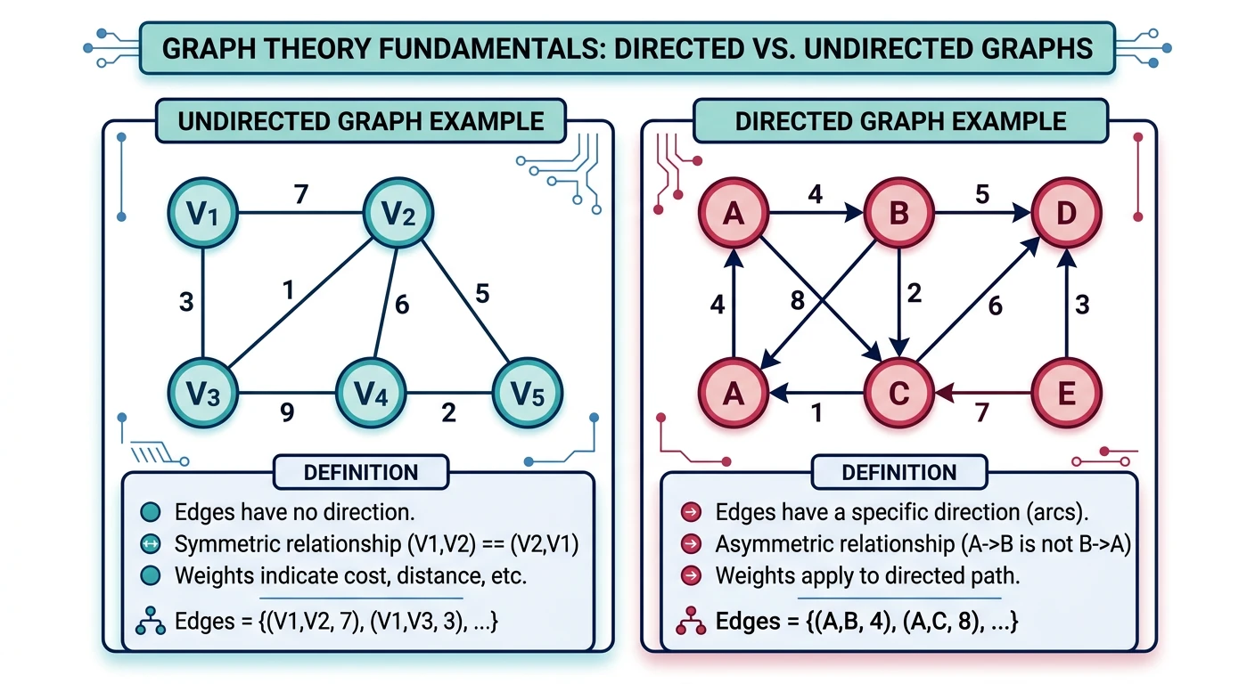
A Graph is a collection of nodes (vertices) and edges connecting them. Graphs model relationships and networks, appearing frequently in interview problems.

Directed and undirected graph examples with vertices, edges, and weights labeled — Graph types: undirected graph with bidirectional edges, directed graph with one-way edges, and weighted graph with edge costs

                            Graph Terminology
                            Directed: Edges have direction (A?B)
Undirected: Edges go both ways (A—B)
Weighted: Edges have costs/weights
Cycle: Path that starts and ends at same node
Connected: Path exists between all vertex pairs

                        

Graph Representations

Choosing the right representation determines the efficiency of every graph algorithm. The Adjacency List maps each vertex to a list of its neighbors — space-efficient for sparse graphs (\(O(V + E)\) space) and fast neighbor iteration. It's the default choice for most interview and production scenarios.

from collections import defaultdict

# 1. Adjacency List (most common for sparse graphs)
class GraphAdjList:
    """
    Adjacency List representation
    Space: O(V + E)
    Best for: sparse graphs, most interview problems
    """
    def __init__(self, directed=False):
        self.graph = defaultdict(list)
        self.directed = directed
    
    def add_edge(self, u, v, weight=1):
        self.graph[u].append((v, weight))
        if not self.directed:
            self.graph[v].append((u, weight))
    
    def get_neighbors(self, u):
        return self.graph[u]
    
    def __str__(self):
        return str(dict(self.graph))

# Example
g = GraphAdjList(directed=False)
g.add_edge(0, 1)
g.add_edge(0, 2)
g.add_edge(1, 2)
g.add_edge(2, 3)

print("Adjacency List:", g)
print("Neighbors of 0:", g.get_neighbors(0))

// Graph Adjacency List - O(V + E) space
#include <vector>
#include <unordered_map>
#include <iostream>

class GraphAdjList {
private:
    std::unordered_map<int, std::vector<std::pair<int, int>>> graph;
    bool directed;
    
public:
    GraphAdjList(bool isDirected = false) : directed(isDirected) {}
    
    void addEdge(int u, int v, int weight = 1) {
        graph[u].push_back({v, weight});
        if (!directed) {
            graph[v].push_back({u, weight});
        }
    }
    
    std::vector<std::pair<int, int>>& getNeighbors(int u) {
        return graph[u];
    }
    
    void display() {
        for (auto& [node, neighbors] : graph) {
            std::cout << node << ": ";
            for (auto& [v, w] : neighbors)
                std::cout << "(" << v << "," << w << ") ";
            std::cout << std::endl;
        }
    }
};

// Graph Adjacency List - O(V + E) space
import java.util.*;

class GraphAdjList {
    private Map<Integer, List<int[]>> graph;
    private boolean directed;
    
    public GraphAdjList(boolean directed) {
        this.graph = new HashMap<>();
        this.directed = directed;
    }
    
    public void addEdge(int u, int v, int weight) {
        graph.computeIfAbsent(u, k -> new ArrayList<>()).add(new int[]{v, weight});
        if (!directed) {
            graph.computeIfAbsent(v, k -> new ArrayList<>()).add(new int[]{u, weight});
        }
    }
    
    public void addEdge(int u, int v) { addEdge(u, v, 1); }
    
    public List<int[]> getNeighbors(int u) {
        return graph.getOrDefault(u, new ArrayList<>());
    }
}

The Adjacency Matrix stores a \(V \times V\) boolean/weight matrix where entry \([i][j]\) indicates an edge from \(i\) to \(j\). It enables \(O(1)\) edge existence checks and is ideal for dense graphs (where \(E \approx V^2\)) or algorithms like Floyd-Warshall that iterate over all pairs. The tradeoff is \(O(V^2)\) space regardless of actual edge count.

import numpy as np

# 2. Adjacency Matrix (good for dense graphs)
class GraphAdjMatrix:
    """
    Adjacency Matrix representation
    Space: O(V²)
    Best for: dense graphs, quick edge lookups
    """
    def __init__(self, num_vertices):
        self.V = num_vertices
        self.matrix = [[0] * num_vertices for _ in range(num_vertices)]
    
    def add_edge(self, u, v, weight=1):
        self.matrix[u][v] = weight
        self.matrix[v][u] = weight  # For undirected
    
    def has_edge(self, u, v):
        return self.matrix[u][v] != 0
    
    def get_neighbors(self, u):
        return [v for v in range(self.V) if self.matrix[u][v] != 0]
    
    def display(self):
        for row in self.matrix:
            print(row)

# Example
g = GraphAdjMatrix(4)
g.add_edge(0, 1)
g.add_edge(0, 2)
g.add_edge(1, 2)
g.add_edge(2, 3)

print("Adjacency Matrix:")
g.display()
print("Neighbors of 2:", g.get_neighbors(2))

// Graph Adjacency Matrix - O(V²) space
#include <vector>
#include <iostream>

class GraphAdjMatrix {
private:
    int V;
    std::vector<std::vector<int>> matrix;
    
public:
    GraphAdjMatrix(int numVertices) : V(numVertices), matrix(V, std::vector<int>(V, 0)) {}
    
    void addEdge(int u, int v, int weight = 1) {
        matrix[u][v] = weight;
        matrix[v][u] = weight;  // Undirected
    }
    
    bool hasEdge(int u, int v) { return matrix[u][v] != 0; }
    
    std::vector<int> getNeighbors(int u) {
        std::vector<int> neighbors;
        for (int v = 0; v < V; v++)
            if (matrix[u][v] != 0) neighbors.push_back(v);
        return neighbors;
    }
    
    void display() {
        for (auto& row : matrix) {
            for (int val : row) std::cout << val << " ";
            std::cout << std::endl;
        }
    }
};

// Graph Adjacency Matrix - O(V²) space
import java.util.*;

class GraphAdjMatrix {
    private int V;
    private int[][] matrix;
    
    public GraphAdjMatrix(int numVertices) {
        V = numVertices;
        matrix = new int[V][V];
    }
    
    public void addEdge(int u, int v, int weight) {
        matrix[u][v] = weight;
        matrix[v][u] = weight;  // Undirected
    }
    
    public void addEdge(int u, int v) { addEdge(u, v, 1); }
    
    public boolean hasEdge(int u, int v) { return matrix[u][v] != 0; }
    
    public List<Integer> getNeighbors(int u) {
        List<Integer> neighbors = new ArrayList<>();
        for (int v = 0; v < V; v++)
            if (matrix[u][v] != 0) neighbors.add(v);
        return neighbors;
    }
}

The Edge List is the simplest representation: just a flat list of \((u, v, weight)\) tuples. It's optimal for algorithms that iterate over all edges (Bellman-Ford, Kruskal's MST) and uses \(O(E)\) space. However, finding neighbors of a specific vertex requires \(O(E)\) scan, making it unsuitable for BFS/DFS.

# 3. Edge List (simplest representation)
class GraphEdgeList:
    """
    Edge List representation
    Space: O(E)
    Best for: algorithms that iterate over all edges
    """
    def __init__(self):
        self.edges = []
    
    def add_edge(self, u, v, weight=1):
        self.edges.append((u, v, weight))
    
    def get_edges(self):
        return self.edges

# Example
g = GraphEdgeList()
g.add_edge(0, 1, 4)
g.add_edge(0, 2, 2)
g.add_edge(1, 2, 1)
g.add_edge(2, 3, 5)

print("Edge List:", g.get_edges())

// Graph Edge List - O(E) space
#include <vector>
#include <tuple>

class GraphEdgeList {
private:
    std::vector<std::tuple<int, int, int>> edges;  // (u, v, weight)
    
public:
    void addEdge(int u, int v, int weight = 1) {
        edges.push_back({u, v, weight});
    }
    
    const std::vector<std::tuple<int, int, int>>& getEdges() {
        return edges;
    }
};

// Graph Edge List - O(E) space
import java.util.*;

class GraphEdgeList {
    private List<int[]> edges;  // {u, v, weight}
    
    public GraphEdgeList() { edges = new ArrayList<>(); }
    
    public void addEdge(int u, int v, int weight) {
        edges.add(new int[]{u, v, weight});
    }
    
    public List<int[]> getEdges() { return edges; }
}

BFS & DFS Traversal

BFS level-by-level traversal vs DFS depth-first traversal on the same graph — BFS vs DFS: BFS explores level by level using a queue, DFS explores as deep as possible using a stack or recursion

BFS vs DFS Strategy Selection

                            flowchart TD
                                A["Graph Problem"] --> B{"What do you need?"}
                                B -->|"Shortest path
(unweighted)"| C["BFS"]
                                B -->|"Cycle detection
or exhaustive search"| D["DFS"]
                                B -->|"Shortest path
(weighted, no negatives)"| E["Dijkstra"]
                                B -->|"Shortest path
(negative edges)"| F["Bellman-Ford"]
                                B -->|"Connected
components"| G["BFS or DFS"]
                                B -->|"Topological
ordering"| H["DFS + finish time"]
                                C --> C1["Queue-based
O(V+E) time"]
                                D --> D1["Stack/Recursion
O(V+E) time"]
                                E --> E1["Priority Queue
O((V+E) log V)"]
                                F --> F1["Relax all edges V-1 times
O(V·E)"]

Interactive: BFS vs DFS Traversal

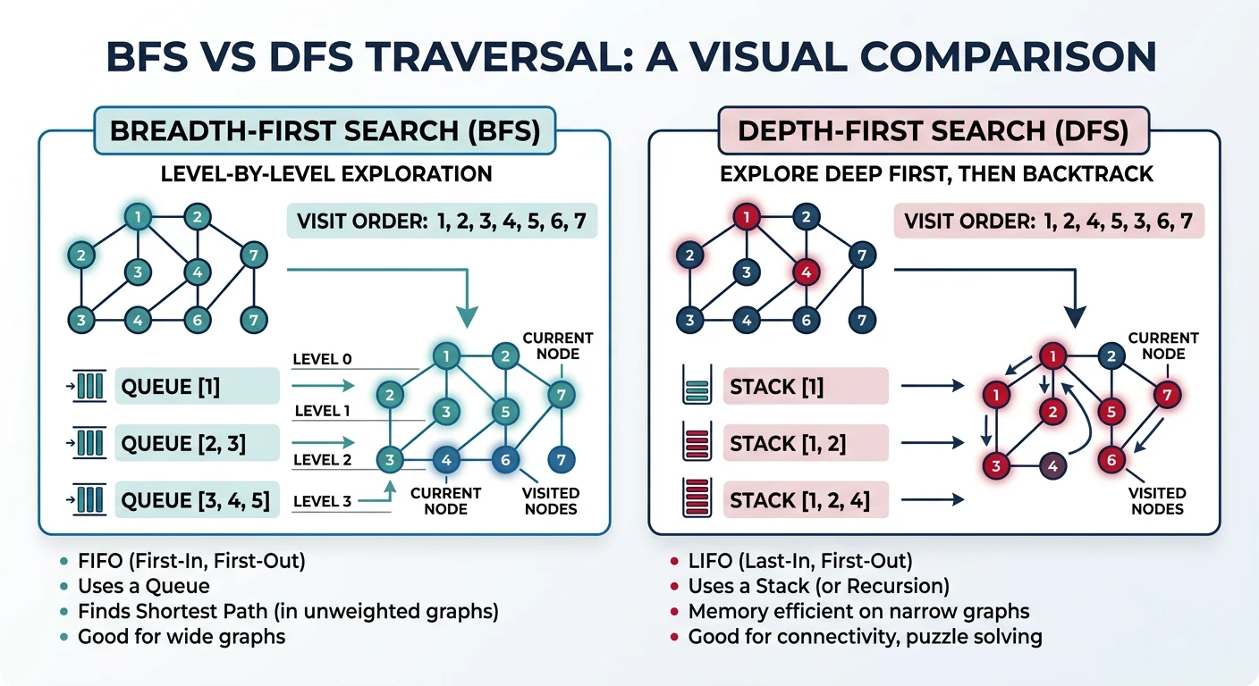
Step through both BFS and DFS on the same graph. Watch how the queue (BFS) explores level-by-level while the stack (DFS) dives deep before backtracking.

BFS vs DFS — Live Comparison

Unvisited Current In Queue/Stack Visited

BFS: Start at Node A

Click Next to step through BFS first, then DFS on the same graph.

Queue: [A] Step 1 / 10

Breadth-First Search (BFS)

BFS explores a graph level by level, visiting all neighbors at distance 1 before any at distance 2, and so on. It uses a queue (FIFO) to maintain the frontier. BFS naturally finds the shortest path in unweighted graphs because it discovers nodes in order of increasing distance from the source. Time: \(O(V + E)\), Space: \(O(V)\) for the visited set and queue.

When to use BFS: shortest path in unweighted graphs, level-order traversal, finding connected components, testing bipartiteness, or any problem where you need to explore "closest first" (like word ladder, minimum mutations, or maze shortest path).

from collections import deque, defaultdict

def bfs(graph, start):
    """
    Breadth-First Search
    Time: O(V + E), Space: O(V)
    Use for: shortest path in unweighted graphs, level-order traversal
    """
    visited = set([start])
    queue = deque([start])
    result = []
    
    while queue:
        node = queue.popleft()
        result.append(node)
        
        for neighbor in graph[node]:
            if neighbor not in visited:
                visited.add(neighbor)
                queue.append(neighbor)
    
    return result

def bfs_shortest_path(graph, start, end):
    """
    BFS for shortest path in unweighted graph
    Returns path from start to end
    """
    if start == end:
        return [start]
    
    visited = {start}
    queue = deque([(start, [start])])
    
    while queue:
        node, path = queue.popleft()
        
        for neighbor in graph[node]:
            if neighbor == end:
                return path + [neighbor]
            
            if neighbor not in visited:
                visited.add(neighbor)
                queue.append((neighbor, path + [neighbor]))
    
    return []  # No path found

# Example
graph = defaultdict(list)
edges = [(0, 1), (0, 2), (1, 2), (1, 3), (2, 3), (3, 4)]
for u, v in edges:
    graph[u].append(v)
    graph[v].append(u)

print("BFS traversal:", bfs(graph, 0))
print("Shortest path 0?4:", bfs_shortest_path(graph, 0, 4))

// BFS Traversal and Shortest Path
#include <vector>
#include <queue>
#include <unordered_set>
#include <unordered_map>

class GraphBFS {
public:
    // BFS traversal - O(V + E) time
    static std::vector<int> bfs(std::unordered_map<int, std::vector<int>>& graph, int start) {
        std::vector<int> result;
        std::unordered_set<int> visited;
        std::queue<int> q;
        
        visited.insert(start);
        q.push(start);
        
        while (!q.empty()) {
            int node = q.front(); q.pop();
            result.push_back(node);
            
            for (int neighbor : graph[node]) {
                if (visited.find(neighbor) == visited.end()) {
                    visited.insert(neighbor);
                    q.push(neighbor);
                }
            }
        }
        return result;
    }
    
    // Shortest path in unweighted graph
    static std::vector<int> shortestPath(std::unordered_map<int, std::vector<int>>& graph, int start, int end) {
        if (start == end) return {start};
        
        std::unordered_set<int> visited;
        std::queue<std::pair<int, std::vector<int>>> q;
        
        visited.insert(start);
        q.push({start, {start}});
        
        while (!q.empty()) {
            auto [node, path] = q.front(); q.pop();
            
            for (int neighbor : graph[node]) {
                if (neighbor == end) {
                    path.push_back(neighbor);
                    return path;
                }
                if (visited.find(neighbor) == visited.end()) {
                    visited.insert(neighbor);
                    std::vector<int> newPath = path;
                    newPath.push_back(neighbor);
                    q.push({neighbor, newPath});
                }
            }
        }
        return {};  // No path
    }
};

// BFS Traversal and Shortest Path
import java.util.*;

class GraphBFS {
    // BFS traversal - O(V + E) time
    public static List<Integer> bfs(Map<Integer, List<Integer>> graph, int start) {
        List<Integer> result = new ArrayList<>();
        Set<Integer> visited = new HashSet<>();
        Queue<Integer> queue = new LinkedList<>();
        
        visited.add(start);
        queue.offer(start);
        
        while (!queue.isEmpty()) {
            int node = queue.poll();
            result.add(node);
            
            for (int neighbor : graph.getOrDefault(node, new ArrayList<>())) {
                if (!visited.contains(neighbor)) {
                    visited.add(neighbor);
                    queue.offer(neighbor);
                }
            }
        }
        return result;
    }
    
    // Shortest path in unweighted graph
    public static List<Integer> shortestPath(Map<Integer, List<Integer>> graph, int start, int end) {
        if (start == end) return Arrays.asList(start);
        
        Set<Integer> visited = new HashSet<>();
        Queue<List<Integer>> queue = new LinkedList<>();
        
        visited.add(start);
        queue.offer(new ArrayList<>(Arrays.asList(start)));
        
        while (!queue.isEmpty()) {
            List<Integer> path = queue.poll();
            int node = path.get(path.size() - 1);
            
            for (int neighbor : graph.getOrDefault(node, new ArrayList<>())) {
                if (neighbor == end) {
                    path.add(neighbor);
                    return path;
                }
                if (!visited.contains(neighbor)) {
                    visited.add(neighbor);
                    List<Integer> newPath = new ArrayList<>(path);
                    newPath.add(neighbor);
                    queue.offer(newPath);
                }
            }
        }
        return new ArrayList<>();  // No path
    }
}

Depth-First Search (DFS)

DFS explores as deep as possible along each branch before backtracking. It uses a stack (explicit or via recursion's call stack). DFS is the natural choice for problems requiring exhaustive exploration: detecting cycles, topological sorting, finding connected/strongly-connected components, and solving puzzles (mazes, Sudoku). Time: \(O(V + E)\), Space: \(O(V)\) for the visited set plus \(O(h)\) stack depth.

Recursive vs Iterative: Recursive DFS is cleaner for tree-like structures, but risks stack overflow on deep graphs (100K+ nodes). Iterative DFS with an explicit stack handles arbitrary depth safely.

from collections import defaultdict

def dfs_recursive(graph, start, visited=None):
    """
    DFS - Recursive implementation
    Time: O(V + E), Space: O(V) for call stack
    """
    if visited is None:
        visited = set()
    
    visited.add(start)
    result = [start]
    
    for neighbor in graph[start]:
        if neighbor not in visited:
            result.extend(dfs_recursive(graph, neighbor, visited))
    
    return result

def dfs_iterative(graph, start):
    """
    DFS - Iterative implementation using stack
    Time: O(V + E), Space: O(V)
    """
    visited = set()
    stack = [start]
    result = []
    
    while stack:
        node = stack.pop()
        
        if node not in visited:
            visited.add(node)
            result.append(node)
            
            # Add neighbors in reverse order for consistent ordering
            for neighbor in reversed(graph[node]):
                if neighbor not in visited:
                    stack.append(neighbor)
    
    return result

# Example
graph = defaultdict(list)
edges = [(0, 1), (0, 2), (1, 3), (1, 4), (2, 5)]
for u, v in edges:
    graph[u].append(v)
    graph[v].append(u)

print("DFS recursive:", dfs_recursive(graph, 0))
print("DFS iterative:", dfs_iterative(graph, 0))

// DFS Traversal - Recursive and Iterative
#include <vector>
#include <stack>
#include <unordered_set>
#include <unordered_map>

class GraphDFS {
public:
    // DFS recursive
    static std::vector<int> dfsRecursive(std::unordered_map<int, std::vector<int>>& graph, 
                                          int node, std::unordered_set<int>& visited) {
        std::vector<int> result;
        visited.insert(node);
        result.push_back(node);
        
        for (int neighbor : graph[node]) {
            if (visited.find(neighbor) == visited.end()) {
                auto subResult = dfsRecursive(graph, neighbor, visited);
                result.insert(result.end(), subResult.begin(), subResult.end());
            }
        }
        return result;
    }
    
    // DFS iterative
    static std::vector<int> dfsIterative(std::unordered_map<int, std::vector<int>>& graph, int start) {
        std::vector<int> result;
        std::unordered_set<int> visited;
        std::stack<int> stk;
        
        stk.push(start);
        
        while (!stk.empty()) {
            int node = stk.top(); stk.pop();
            
            if (visited.find(node) == visited.end()) {
                visited.insert(node);
                result.push_back(node);
                
                // Add neighbors in reverse for consistent order
                auto& neighbors = graph[node];
                for (auto it = neighbors.rbegin(); it != neighbors.rend(); ++it) {
                    if (visited.find(*it) == visited.end())
                        stk.push(*it);
                }
            }
        }
        return result;
    }
};

// DFS Traversal - Recursive and Iterative
import java.util.*;

class GraphDFS {
    // DFS recursive
    public static void dfsRecursive(Map<Integer, List<Integer>> graph, int node,
                                     Set<Integer> visited, List<Integer> result) {
        visited.add(node);
        result.add(node);
        
        for (int neighbor : graph.getOrDefault(node, new ArrayList<>())) {
            if (!visited.contains(neighbor)) {
                dfsRecursive(graph, neighbor, visited, result);
            }
        }
    }
    
    // DFS iterative
    public static List<Integer> dfsIterative(Map<Integer, List<Integer>> graph, int start) {
        List<Integer> result = new ArrayList<>();
        Set<Integer> visited = new HashSet<>();
        Deque<Integer> stack = new ArrayDeque<>();
        
        stack.push(start);
        
        while (!stack.isEmpty()) {
            int node = stack.pop();
            
            if (!visited.contains(node)) {
                visited.add(node);
                result.add(node);
                
                List<Integer> neighbors = graph.getOrDefault(node, new ArrayList<>());
                for (int i = neighbors.size() - 1; i >= 0; i--) {
                    if (!visited.contains(neighbors.get(i)))
                        stack.push(neighbors.get(i));
                }
            }
        }
        return result;
    }
}

Number of Islands (Classic Graph Problem)

Given a 2D grid of '1's (land) and '0's (water), count the number of islands. An island is surrounded by water and formed by connecting adjacent lands horizontally or vertically. This is the canonical flood-fill / connected components problem: scan the grid; when you hit unvisited land, start a DFS/BFS to mark the entire island as visited, then increment the count. Each cell is visited at most once, giving \(O(m \times n)\) time.

def num_islands(grid):
    """
    LeetCode 200: Number of Islands
    Time: O(m*n), Space: O(m*n) for recursion
    """
    if not grid:
        return 0
    
    rows, cols = len(grid), len(grid[0])
    count = 0
    
    def dfs(r, c):
        # Boundary check and water/visited check
        if (r < 0 or r >= rows or 
            c < 0 or c >= cols or 
            grid[r][c] != '1'):
            return
        
        # Mark as visited
        grid[r][c] = '#'
        
        # Explore all 4 directions
        dfs(r + 1, c)
        dfs(r - 1, c)
        dfs(r, c + 1)
        dfs(r, c - 1)
    
    for r in range(rows):
        for c in range(cols):
            if grid[r][c] == '1':
                count += 1
                dfs(r, c)
    
    return count

# Example
grid = [
    ['1', '1', '0', '0', '0'],
    ['1', '1', '0', '0', '0'],
    ['0', '0', '1', '0', '0'],
    ['0', '0', '0', '1', '1']
]

print("Number of islands:", num_islands(grid))  # 3

// LeetCode 200: Number of Islands
// Time: O(m*n), Space: O(m*n)
#include <vector>

class NumIslands {
public:
    int numIslands(std::vector<std::vector<char>>& grid) {
        if (grid.empty()) return 0;
        
        int rows = grid.size(), cols = grid[0].size();
        int count = 0;
        
        for (int r = 0; r < rows; r++) {
            for (int c = 0; c < cols; c++) {
                if (grid[r][c] == '1') {
                    count++;
                    dfs(grid, r, c, rows, cols);
                }
            }
        }
        return count;
    }
    
private:
    void dfs(std::vector<std::vector<char>>& grid, int r, int c, int rows, int cols) {
        if (r < 0 || r >= rows || c < 0 || c >= cols || grid[r][c] != '1')
            return;
        
        grid[r][c] = '#';  // Mark visited
        dfs(grid, r + 1, c, rows, cols);
        dfs(grid, r - 1, c, rows, cols);
        dfs(grid, r, c + 1, rows, cols);
        dfs(grid, r, c - 1, rows, cols);
    }
};

// LeetCode 200: Number of Islands
// Time: O(m*n), Space: O(m*n)

class NumIslands {
    public int numIslands(char[][] grid) {
        if (grid == null || grid.length == 0) return 0;
        
        int rows = grid.length, cols = grid[0].length;
        int count = 0;
        
        for (int r = 0; r < rows; r++) {
            for (int c = 0; c < cols; c++) {
                if (grid[r][c] == '1') {
                    count++;
                    dfs(grid, r, c, rows, cols);
                }
            }
        }
        return count;
    }
    
    private void dfs(char[][] grid, int r, int c, int rows, int cols) {
        if (r < 0 || r >= rows || c < 0 || c >= cols || grid[r][c] != '1')
            return;
        
        grid[r][c] = '#';  // Mark visited
        dfs(grid, r + 1, c, rows, cols);
        dfs(grid, r - 1, c, rows, cols);
        dfs(grid, r, c + 1, rows, cols);
        dfs(grid, r, c - 1, rows, cols);
    }
}

Shortest Path Algorithms

Dijkstra algorithm step-by-step showing priority queue processing and distance updates — Dijkstra's algorithm: greedily select the nearest unvisited vertex, update neighbor distances, and repeat until all vertices are processed

Shortest Path Algorithm Selection

flowchart TD
    A["Shortest Path Problem"] --> B{"Negative
Weights?"}
    B -->|No| C{"Single Source?"}
    B -->|Yes| D{"Negative
Cycles?"}

    C -->|Yes| E{"Weighted?"}
    C -->|No| F["Floyd-Warshall
O V cubed"]

    E -->|Yes| G["Dijkstra
O V+E log V"]
    E -->|No| H["BFS
O V+E"]

    D -->|No| I["Bellman-Ford
O VE"]
    D -->|Yes| J["No Solution
Detect and Report"]

    style G fill:#e8f4f4,stroke:#3B9797
    style H fill:#e8f4f4,stroke:#3B9797
    style I fill:#f0f4f8,stroke:#16476A
    style J fill:#fff5f5,stroke:#BF092F

Dijkstra's Algorithm

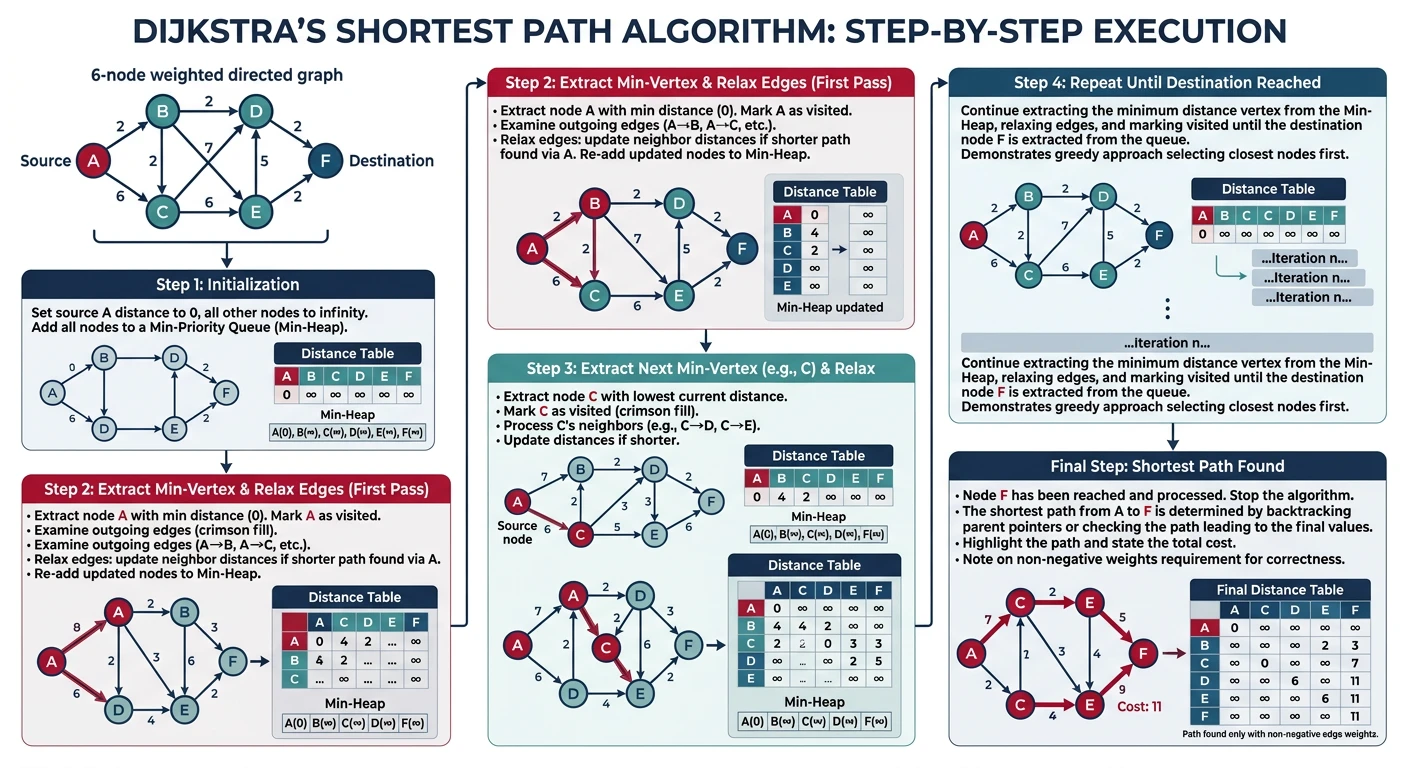
Dijkstra's algorithm finds the shortest path from a single source vertex to all other vertices in a graph with non-negative edge weights. It works on a greedy principle: always process the unvisited vertex with the smallest known distance, then update its neighbors. This greedy choice is safe because non-negative weights guarantee that once a vertex is finalized (popped from the priority queue), no shorter path to it can exist.

Key Insight

Think of Dijkstra as a "wavefront" expanding outward from the source — it always expands to the nearest unvisited node first, like ripples on a pond. The priority queue (min-heap) efficiently selects which node to expand next. Time complexity: \(O((V + E) \log V)\) with a binary heap.

Algorithm steps: (1) Initialize all distances to ∞ except source = 0. (2) Push source into a min-heap. (3) Pop the minimum-distance vertex, relax all its edges (if \(dist[u] + weight(u,v) < dist[v]\), update \(dist[v]\)). (4) Repeat until the heap is empty. The relaxation step is the core — it asks "can we reach \(v\) faster by going through \(u\)?"

import heapq
from collections import defaultdict

def dijkstra(graph, start):
    """
    Dijkstra's Algorithm for shortest paths
    Time: O((V + E) log V), Space: O(V)
    Works for non-negative weights only
    """
    # Distance to all nodes (infinity initially)
    distances = {node: float('inf') for node in graph}
    distances[start] = 0
    
    # Priority queue: (distance, node)
    pq = [(0, start)]
    
    # Track visited nodes
    visited = set()
    
    while pq:
        dist, node = heapq.heappop(pq)
        
        if node in visited:
            continue
        
        visited.add(node)
        
        for neighbor, weight in graph[node]:
            if neighbor not in visited:
                new_dist = dist + weight
                
                if new_dist < distances[neighbor]:
                    distances[neighbor] = new_dist
                    heapq.heappush(pq, (new_dist, neighbor))
    
    return distances

# Example: Weighted graph
graph = defaultdict(list)
edges = [
    (0, 1, 4), (0, 2, 1),
    (1, 3, 1),
    (2, 1, 2), (2, 3, 5),
    (3, 4, 3)
]

for u, v, w in edges:
    graph[u].append((v, w))

distances = dijkstra(graph, 0)
print("Shortest distances from 0:")
for node, dist in sorted(distances.items()):
    print(f"  To {node}: {dist}")

// Dijkstra's Algorithm - O((V + E) log V)
// Non-negative weights only
#include <vector>
#include <queue>
#include <unordered_map>
#include <limits>

class Dijkstra {
public:
    static std::unordered_map<int, int> shortestPaths(
            std::unordered_map<int, std::vector<std::pair<int, int>>>& graph, int start) {
        
        std::unordered_map<int, int> distances;
        for (auto& [node, _] : graph)
            distances[node] = std::numeric_limits<int>::max();
        distances[start] = 0;
        
        // Min heap: (distance, node)
        std::priority_queue<std::pair<int, int>, std::vector<std::pair<int, int>>,
                           std::greater<>> pq;
        pq.push({0, start});
        
        std::unordered_set<int> visited;
        
        while (!pq.empty()) {
            auto [dist, node] = pq.top(); pq.pop();
            
            if (visited.count(node)) continue;
            visited.insert(node);
            
            for (auto& [neighbor, weight] : graph[node]) {
                int newDist = dist + weight;
                if (newDist < distances[neighbor]) {
                    distances[neighbor] = newDist;
                    pq.push({newDist, neighbor});
                }
            }
        }
        return distances;
    }
};

// Dijkstra's Algorithm - O((V + E) log V)
// Non-negative weights only
import java.util.*;

class Dijkstra {
    public static Map<Integer, Integer> shortestPaths(
            Map<Integer, List<int[]>> graph, int start) {
        
        Map<Integer, Integer> distances = new HashMap<>();
        for (int node : graph.keySet())
            distances.put(node, Integer.MAX_VALUE);
        distances.put(start, 0);
        
        // Min heap: {distance, node}
        PriorityQueue<int[]> pq = new PriorityQueue<>((a, b) -> a[0] - b[0]);
        pq.offer(new int[]{0, start});
        
        Set<Integer> visited = new HashSet<>();
        
        while (!pq.isEmpty()) {
            int[] curr = pq.poll();
            int dist = curr[0], node = curr[1];
            
            if (visited.contains(node)) continue;
            visited.add(node);
            
            for (int[] edge : graph.getOrDefault(node, new ArrayList<>())) {
                int neighbor = edge[0], weight = edge[1];
                int newDist = dist + weight;
                if (newDist < distances.getOrDefault(neighbor, Integer.MAX_VALUE)) {
                    distances.put(neighbor, newDist);
                    pq.offer(new int[]{newDist, neighbor});
                }
            }
        }
        return distances;
    }
}

Bellman-Ford Algorithm

Bellman-Ford solves the single-source shortest path problem even when edges have negative weights — something Dijkstra cannot handle. The tradeoff is speed: \(O(V \times E)\) versus Dijkstra's \(O((V+E) \log V)\). Its key advantage is the ability to detect negative-weight cycles — loops where total weight is negative, making "shortest path" undefined (you could loop forever getting shorter).

How it works: Relax every edge in the graph \(V-1\) times. After \(k\) iterations, the algorithm guarantees correct shortest distances for all paths using at most \(k\) edges. Since the longest simple path has at most \(V-1\) edges, \(V-1\) iterations suffice. If a \(V\)-th iteration still reduces a distance, a negative cycle exists.

When to Choose Bellman-Ford over Dijkstra

Use Bellman-Ford when: (1) edges can have negative weights (e.g., currency arbitrage, network routing with costs/rebates), (2) you need to detect negative cycles, or (3) the graph is given as an edge list (Bellman-Ford iterates over edges directly). For all other cases, prefer Dijkstra for speed.

def bellman_ford(vertices, edges, start):
    """
    Bellman-Ford Algorithm
    Time: O(V * E), Space: O(V)
    Handles negative weights, detects negative cycles
    """
    # Initialize distances
    distances = {v: float('inf') for v in vertices}
    distances[start] = 0
    
    # Relax edges V-1 times
    for _ in range(len(vertices) - 1):
        for u, v, weight in edges:
            if distances[u] != float('inf'):
                if distances[u] + weight < distances[v]:
                    distances[v] = distances[u] + weight
    
    # Check for negative cycles
    for u, v, weight in edges:
        if distances[u] != float('inf'):
            if distances[u] + weight < distances[v]:
                return None  # Negative cycle detected
    
    return distances

# Example
vertices = [0, 1, 2, 3, 4]
edges = [
    (0, 1, 4), (0, 2, 1),
    (1, 3, 1),
    (2, 1, 2), (2, 3, 5),
    (3, 4, 3)
]

distances = bellman_ford(vertices, edges, 0)
print("Bellman-Ford distances from 0:")
for node, dist in sorted(distances.items()):
    print(f"  To {node}: {dist}")

// Bellman-Ford Algorithm - O(V * E)
// Handles negative weights, detects negative cycles
#include <vector>
#include <limits>
#include <unordered_map>

class BellmanFord {
public:
    static std::unordered_map<int, int> shortestPaths(
            std::vector<int>& vertices,
            std::vector<std::tuple<int, int, int>>& edges, int start) {
        
        std::unordered_map<int, int> distances;
        for (int v : vertices)
            distances[v] = std::numeric_limits<int>::max();
        distances[start] = 0;
        
        // Relax edges V-1 times
        for (int i = 0; i < vertices.size() - 1; i++) {
            for (auto& [u, v, weight] : edges) {
                if (distances[u] != std::numeric_limits<int>::max() &&
                    distances[u] + weight < distances[v]) {
                    distances[v] = distances[u] + weight;
                }
            }
        }
        
        // Check for negative cycles
        for (auto& [u, v, weight] : edges) {
            if (distances[u] != std::numeric_limits<int>::max() &&
                distances[u] + weight < distances[v]) {
                return {};  // Negative cycle detected
            }
        }
        
        return distances;
    }
};

// Bellman-Ford Algorithm - O(V * E)
// Handles negative weights, detects negative cycles
import java.util.*;

class BellmanFord {
    public static Map<Integer, Integer> shortestPaths(
            int[] vertices, int[][] edges, int start) {
        
        Map<Integer, Integer> distances = new HashMap<>();
        for (int v : vertices)
            distances.put(v, Integer.MAX_VALUE);
        distances.put(start, 0);
        
        // Relax edges V-1 times
        for (int i = 0; i < vertices.length - 1; i++) {
            for (int[] edge : edges) {
                int u = edge[0], v = edge[1], weight = edge[2];
                if (distances.get(u) != Integer.MAX_VALUE &&
                    distances.get(u) + weight < distances.get(v)) {
                    distances.put(v, distances.get(u) + weight);
                }
            }
        }
        
        // Check for negative cycles
        for (int[] edge : edges) {
            int u = edge[0], v = edge[1], weight = edge[2];
            if (distances.get(u) != Integer.MAX_VALUE &&
                distances.get(u) + weight < distances.get(v)) {
                return null;  // Negative cycle detected
            }
        }
        
        return distances;
    }
}

Topological Sort

A topological ordering of a Directed Acyclic Graph (DAG) arranges vertices so that for every directed edge \(u \to v\), vertex \(u\) appears before \(v\). Think of it as a valid execution order — like determining which courses to take first given prerequisites, or which build targets to compile before others.

Two classic approaches exist: Kahn's Algorithm (BFS-based) repeatedly removes vertices with zero in-degree, while the DFS-based approach adds vertices to the result in reverse post-order. Both run in \(O(V + E)\). A topological sort exists if and only if the graph has no cycles — if Kahn's algorithm processes fewer than \(V\) vertices, a cycle exists.

Real-World Applications

Build systems (Makefile dependencies), package managers (npm/pip install order), spreadsheet cell evaluation (formulas depend on other cells), course scheduling (prerequisites), and task pipelines (CI/CD stages). Any problem with "do X before Y" constraints maps to topological sort.

from collections import deque, defaultdict

def topological_sort_kahn(num_nodes, edges):
    """
    Kahn's Algorithm (BFS-based)
    Time: O(V + E), Space: O(V)
    Returns topological order or empty list if cycle exists
    """
    # Build graph and compute in-degrees
    graph = defaultdict(list)
    in_degree = [0] * num_nodes
    
    for u, v in edges:
        graph[u].append(v)
        in_degree[v] += 1
    
    # Start with nodes having no prerequisites
    queue = deque([i for i in range(num_nodes) if in_degree[i] == 0])
    result = []
    
    while queue:
        node = queue.popleft()
        result.append(node)
        
        for neighbor in graph[node]:
            in_degree[neighbor] -= 1
            if in_degree[neighbor] == 0:
                queue.append(neighbor)
    
    # Check if all nodes are included (no cycle)
    return result if len(result) == num_nodes else []

def topological_sort_dfs(num_nodes, edges):
    """
    DFS-based topological sort
    Time: O(V + E), Space: O(V)
    """
    graph = defaultdict(list)
    for u, v in edges:
        graph[u].append(v)
    
    visited = [0] * num_nodes  # 0: unvisited, 1: visiting, 2: visited
    result = []
    
    def dfs(node):
        if visited[node] == 1:  # Cycle detected
            return False
        if visited[node] == 2:
            return True
        
        visited[node] = 1  # Mark as visiting
        
        for neighbor in graph[node]:
            if not dfs(neighbor):
                return False
        
        visited[node] = 2  # Mark as visited
        result.append(node)
        return True
    
    for i in range(num_nodes):
        if visited[i] == 0:
            if not dfs(i):
                return []  # Cycle detected
    
    return result[::-1]  # Reverse for topological order

# Example: Course Schedule
# 0 -> 1 -> 3
#      |
# 2 ---+
num_courses = 4
prerequisites = [(0, 1), (1, 3), (2, 1)]

print("Topological order (Kahn):", topological_sort_kahn(num_courses, prerequisites))
print("Topological order (DFS):", topological_sort_dfs(num_courses, prerequisites))

// Topological Sort - Kahn's Algorithm (BFS)
// Time: O(V + E), Space: O(V)
#include <vector>
#include <queue>
#include <unordered_map>

class TopologicalSort {
public:
    // Kahn's Algorithm (BFS)
    static std::vector<int> kahnSort(int numNodes, std::vector<std::pair<int, int>>& edges) {
        std::unordered_map<int, std::vector<int>> graph;
        std::vector<int> inDegree(numNodes, 0);
        
        for (auto& [u, v] : edges) {
            graph[u].push_back(v);
            inDegree[v]++;
        }
        
        std::queue<int> q;
        for (int i = 0; i < numNodes; i++)
            if (inDegree[i] == 0) q.push(i);
        
        std::vector<int> result;
        while (!q.empty()) {
            int node = q.front(); q.pop();
            result.push_back(node);
            
            for (int neighbor : graph[node]) {
                if (--inDegree[neighbor] == 0)
                    q.push(neighbor);
            }
        }
        
        return (result.size() == numNodes) ? result : std::vector<int>();
    }
    
    // DFS-based topological sort
    static std::vector<int> dfsSort(int numNodes, std::vector<std::pair<int, int>>& edges) {
        std::unordered_map<int, std::vector<int>> graph;
        for (auto& [u, v] : edges)
            graph[u].push_back(v);
        
        std::vector<int> visited(numNodes, 0);  // 0=unvisited, 1=visiting, 2=visited
        std::vector<int> result;
        
        std::function<bool(int)> dfs = [&](int node) {
            if (visited[node] == 1) return false;  // Cycle
            if (visited[node] == 2) return true;
            
            visited[node] = 1;
            for (int neighbor : graph[node])
                if (!dfs(neighbor)) return false;
            
            visited[node] = 2;
            result.push_back(node);
            return true;
        };
        
        for (int i = 0; i < numNodes; i++)
            if (visited[i] == 0 && !dfs(i)) return {};
        
        std::reverse(result.begin(), result.end());
        return result;
    }
};

// Topological Sort - Kahn's Algorithm (BFS) and DFS
import java.util.*;

class TopologicalSort {
    // Kahn's Algorithm (BFS)
    public static List<Integer> kahnSort(int numNodes, int[][] edges) {
        Map<Integer, List<Integer>> graph = new HashMap<>();
        int[] inDegree = new int[numNodes];
        
        for (int[] edge : edges) {
            graph.computeIfAbsent(edge[0], k -> new ArrayList<>()).add(edge[1]);
            inDegree[edge[1]]++;
        }
        
        Queue<Integer> queue = new LinkedList<>();
        for (int i = 0; i < numNodes; i++)
            if (inDegree[i] == 0) queue.offer(i);
        
        List<Integer> result = new ArrayList<>();
        while (!queue.isEmpty()) {
            int node = queue.poll();
            result.add(node);
            
            for (int neighbor : graph.getOrDefault(node, new ArrayList<>())) {
                if (--inDegree[neighbor] == 0)
                    queue.offer(neighbor);
            }
        }
        
        return (result.size() == numNodes) ? result : new ArrayList<>();
    }
    
    // DFS-based topological sort
    public static List<Integer> dfsSort(int numNodes, int[][] edges) {
        Map<Integer, List<Integer>> graph = new HashMap<>();
        for (int[] edge : edges)
            graph.computeIfAbsent(edge[0], k -> new ArrayList<>()).add(edge[1]);
        
        int[] visited = new int[numNodes];  // 0=unvisited, 1=visiting, 2=visited
        List<Integer> result = new ArrayList<>();
        
        for (int i = 0; i < numNodes; i++)
            if (visited[i] == 0 && !dfs(graph, i, visited, result))
                return new ArrayList<>();
        
        Collections.reverse(result);
        return result;
    }
    
    private static boolean dfs(Map<Integer, List<Integer>> graph, int node,
                               int[] visited, List<Integer> result) {
        if (visited[node] == 1) return false;  // Cycle
        if (visited[node] == 2) return true;
        
        visited[node] = 1;
        for (int neighbor : graph.getOrDefault(node, new ArrayList<>()))
            if (!dfs(graph, neighbor, visited, result)) return false;
        
        visited[node] = 2;
        result.add(node);
        return true;
    }
}

Dynamic Programming Introduction

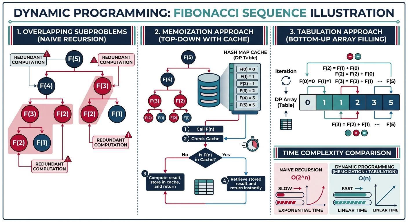
Dynamic Programming (DP) solves problems by breaking them into overlapping subproblems, storing solutions to avoid recomputation. It's essential for optimization problems.

Fibonacci recursion tree showing overlapping subproblems highlighted and memoization table — Dynamic programming illustrated with Fibonacci: recursion tree reveals overlapping subproblems, memoization eliminates redundant computation

                            DP Characteristics
                            Optimal Substructure: Optimal solution contains optimal solutions to subproblems
Overlapping Subproblems: Same subproblems solved multiple times
Memoization: Top-down approach with caching
Tabulation: Bottom-up approach building solution iteratively

                        

DP vs Greedy vs Backtracking Decision Guide

                            flowchart TD
                                A["Optimization Problem"] --> B{"Overlapping
subproblems?"}
                                B -->|"Yes"| C{"Optimal
substructure?"}
                                B -->|"No"| D{"Greedy choice
property?"}
                                C -->|"Yes"| E["Dynamic Programming"]
                                C -->|"No"| F["Backtracking / Brute Force"]
                                D -->|"Yes"| G["Greedy Algorithm"]
                                D -->|"No"| F
                                E --> E1["Top-down: Memoization"]
                                E --> E2["Bottom-up: Tabulation"]
                                G --> G1["Make locally optimal
choice at each step"]
                                F --> F1["Explore all possibilities
with pruning"]

Fibonacci - DP Example

def fib_recursive(n):
    """
    Naive recursive - O(2^n) time!
    """
    if n <= 1:
        return n
    return fib_recursive(n-1) + fib_recursive(n-2)

def fib_memoization(n, memo=None):
    """
    Top-down with memoization - O(n) time, O(n) space
    """
    if memo is None:
        memo = {}
    
    if n in memo:
        return memo[n]
    
    if n <= 1:
        return n
    
    memo[n] = fib_memoization(n-1, memo) + fib_memoization(n-2, memo)
    return memo[n]

def fib_tabulation(n):
    """
    Bottom-up tabulation - O(n) time, O(n) space
    """
    if n <= 1:
        return n
    
    dp = [0] * (n + 1)
    dp[1] = 1
    
    for i in range(2, n + 1):
        dp[i] = dp[i-1] + dp[i-2]
    
    return dp[n]

def fib_optimized(n):
    """
    Space-optimized - O(n) time, O(1) space
    """
    if n <= 1:
        return n
    
    prev2, prev1 = 0, 1
    
    for _ in range(2, n + 1):
        curr = prev1 + prev2
        prev2 = prev1
        prev1 = curr
    
    return prev1

# Compare all approaches
n = 30
print(f"Fibonacci({n}):")
print(f"  Memoization: {fib_memoization(n)}")
print(f"  Tabulation: {fib_tabulation(n)}")
print(f"  Optimized: {fib_optimized(n)}")

// Fibonacci - DP Approaches
#include <vector>
#include <unordered_map>

class Fibonacci {
public:
    // Top-down with memoization - O(n) time, O(n) space
    static int memoization(int n, std::unordered_map<int, int>& memo) {
        if (n <= 1) return n;
        if (memo.count(n)) return memo[n];
        return memo[n] = memoization(n - 1, memo) + memoization(n - 2, memo);
    }
    
    // Bottom-up tabulation - O(n) time, O(n) space
    static int tabulation(int n) {
        if (n <= 1) return n;
        std::vector<int> dp(n + 1);
        dp[0] = 0; dp[1] = 1;
        for (int i = 2; i <= n; i++)
            dp[i] = dp[i-1] + dp[i-2];
        return dp[n];
    }
    
    // Space-optimized - O(n) time, O(1) space
    static int optimized(int n) {
        if (n <= 1) return n;
        int prev2 = 0, prev1 = 1;
        for (int i = 2; i <= n; i++) {
            int curr = prev1 + prev2;
            prev2 = prev1;
            prev1 = curr;
        }
        return prev1;
    }
};

// Fibonacci - DP Approaches
import java.util.*;

class Fibonacci {
    // Top-down with memoization - O(n) time, O(n) space
    public static int memoization(int n, Map<Integer, Integer> memo) {
        if (n <= 1) return n;
        if (memo.containsKey(n)) return memo.get(n);
        int result = memoization(n - 1, memo) + memoization(n - 2, memo);
        memo.put(n, result);
        return result;
    }
    
    // Bottom-up tabulation - O(n) time, O(n) space
    public static int tabulation(int n) {
        if (n <= 1) return n;
        int[] dp = new int[n + 1];
        dp[0] = 0; dp[1] = 1;
        for (int i = 2; i <= n; i++)
            dp[i] = dp[i-1] + dp[i-2];
        return dp[n];
    }
    
    // Space-optimized - O(n) time, O(1) space
    public static int optimized(int n) {
        if (n <= 1) return n;
        int prev2 = 0, prev1 = 1;
        for (int i = 2; i <= n; i++) {
            int curr = prev1 + prev2;
            prev2 = prev1;
            prev1 = curr;
        }
        return prev1;
    }
}

Common DP Patterns

DP problems fall into recognizable families based on the shape of their state space. 1D DP uses a single variable (array index, amount remaining, step count). 2D DP uses two variables (two string indices, grid coordinates, item × capacity). Recognizing the pattern lets you define the recurrence immediately.

1D DP: Climbing Stairs

You can climb 1 or 2 steps at a time. How many distinct ways to reach step \(n\)? This is structurally identical to Fibonacci: \(dp[i] = dp[i-1] + dp[i-2]\). The "number of ways" at each step is the sum of ways to reach it from one step below (1 step) and two steps below (2 steps). State: \(dp[i]\) = ways to reach step \(i\). Transition: \(dp[i] = dp[i-1] + dp[i-2]\). Base: \(dp[0]=1, dp[1]=1\).

def climb_stairs(n):
    """
    LeetCode 70: Climbing Stairs
    Ways to reach top climbing 1 or 2 steps at a time
    Time: O(n), Space: O(1)
    """
    if n <= 2:
        return n
    
    prev2, prev1 = 1, 2
    
    for i in range(3, n + 1):
        curr = prev1 + prev2
        prev2 = prev1
        prev1 = curr
    
    return prev1

# Example
for n in [2, 3, 4, 5]:
    print(f"Ways to climb {n} stairs: {climb_stairs(n)}")

// LeetCode 70: Climbing Stairs
// Time: O(n), Space: O(1)

class ClimbStairs {
public:
    static int climbStairs(int n) {
        if (n <= 2) return n;
        
        int prev2 = 1, prev1 = 2;
        for (int i = 3; i <= n; i++) {
            int curr = prev1 + prev2;
            prev2 = prev1;
            prev1 = curr;
        }
        return prev1;
    }
};

// LeetCode 70: Climbing Stairs
// Time: O(n), Space: O(1)

class ClimbStairs {
    public static int climbStairs(int n) {
        if (n <= 2) return n;
        
        int prev2 = 1, prev1 = 2;
        for (int i = 3; i <= n; i++) {
            int curr = prev1 + prev2;
            prev2 = prev1;
            prev1 = curr;
        }
        return prev1;
    }
}

1D DP: House Robber

Given an array of house values where adjacent houses cannot both be robbed (they trigger an alarm), maximize total loot. This is the classic "include/exclude" DP pattern: at each house \(i\), you either rob it (adding its value to the best from \(i-2\)) or skip it (carrying forward the best from \(i-1\)). State: \(dp[i]\) = max loot from houses \(0..i\). Transition: \(dp[i] = \max(dp[i-1],\; dp[i-2] + nums[i])\). This pattern appears in many variants: circular houses (LeetCode 213), binary tree robber (LeetCode 337).

def house_robber(nums):
    """
    LeetCode 198: House Robber
    Max money robbing non-adjacent houses
    Time: O(n), Space: O(1)
    """
    if not nums:
        return 0
    if len(nums) == 1:
        return nums[0]
    
    # dp[i] = max(rob this house + dp[i-2], skip this house + dp[i-1])
    prev2 = nums[0]
    prev1 = max(nums[0], nums[1])
    
    for i in range(2, len(nums)):
        curr = max(nums[i] + prev2, prev1)
        prev2 = prev1
        prev1 = curr
    
    return prev1

# Example
houses = [2, 7, 9, 3, 1]
print(f"Houses: {houses}")
print(f"Max robbery: {house_robber(houses)}")  # 12 (2 + 9 + 1)

// LeetCode 198: House Robber
// Time: O(n), Space: O(1)
#include <vector>
#include <algorithm>

class HouseRobber {
public:
    static int rob(std::vector<int>& nums) {
        if (nums.empty()) return 0;
        if (nums.size() == 1) return nums[0];
        
        int prev2 = nums[0];
        int prev1 = std::max(nums[0], nums[1]);
        
        for (int i = 2; i < nums.size(); i++) {
            int curr = std::max(nums[i] + prev2, prev1);
            prev2 = prev1;
            prev1 = curr;
        }
        return prev1;
    }
};

// LeetCode 198: House Robber
// Time: O(n), Space: O(1)

class HouseRobber {
    public static int rob(int[] nums) {
        if (nums == null || nums.length == 0) return 0;
        if (nums.length == 1) return nums[0];
        
        int prev2 = nums[0];
        int prev1 = Math.max(nums[0], nums[1]);
        
        for (int i = 2; i < nums.length; i++) {
            int curr = Math.max(nums[i] + prev2, prev1);
            prev2 = prev1;
            prev1 = curr;
        }
        return prev1;
    }
}

2D DP: Longest Common Subsequence

Given two strings, find the length of their longest common subsequence (characters in order but not necessarily contiguous). This is the gateway 2D DP problem — state is defined by two pointers into the two strings. If characters match, both advance; otherwise, try advancing each pointer separately and take the maximum. State: \(dp[i][j]\) = LCS length of \(text1[0..i-1]\) and \(text2[0..j-1]\). Transition: if \(text1[i-1] = text2[j-1]\), then \(dp[i][j] = dp[i-1][j-1] + 1\); else \(dp[i][j] = \max(dp[i-1][j], dp[i][j-1])\).

This pattern generalizes to Edit Distance (add insert/delete/replace costs), Shortest Common Supersequence, and many string-comparison problems.

def longest_common_subsequence(text1, text2):
    """
    LeetCode 1143: Longest Common Subsequence
    Time: O(m*n), Space: O(m*n)
    """
    m, n = len(text1), len(text2)
    
    # dp[i][j] = LCS of text1[0:i] and text2[0:j]
    dp = [[0] * (n + 1) for _ in range(m + 1)]
    
    for i in range(1, m + 1):
        for j in range(1, n + 1):
            if text1[i-1] == text2[j-1]:
                dp[i][j] = dp[i-1][j-1] + 1
            else:
                dp[i][j] = max(dp[i-1][j], dp[i][j-1])
    
    return dp[m][n]

# Example
text1 = "abcde"
text2 = "ace"
print(f"LCS of '{text1}' and '{text2}': {longest_common_subsequence(text1, text2)}")  # 3

// LeetCode 1143: Longest Common Subsequence
// Time: O(m*n), Space: O(m*n)
#include <string>
#include <vector>
#include <algorithm>

class LongestCommonSubsequence {
public:
    static int longestCommonSubsequence(std::string text1, std::string text2) {
        int m = text1.size(), n = text2.size();
        std::vector<std::vector<int>> dp(m + 1, std::vector<int>(n + 1, 0));
        
        for (int i = 1; i <= m; i++) {
            for (int j = 1; j <= n; j++) {
                if (text1[i-1] == text2[j-1])
                    dp[i][j] = dp[i-1][j-1] + 1;
                else
                    dp[i][j] = std::max(dp[i-1][j], dp[i][j-1]);
            }
        }
        return dp[m][n];
    }
};

// LeetCode 1143: Longest Common Subsequence
// Time: O(m*n), Space: O(m*n)

class LongestCommonSubsequence {
    public static int longestCommonSubsequence(String text1, String text2) {
        int m = text1.length(), n = text2.length();
        int[][] dp = new int[m + 1][n + 1];
        
        for (int i = 1; i <= m; i++) {
            for (int j = 1; j <= n; j++) {
                if (text1.charAt(i-1) == text2.charAt(j-1))
                    dp[i][j] = dp[i-1][j-1] + 1;
                else
                    dp[i][j] = Math.max(dp[i-1][j], dp[i][j-1]);
            }
        }
        return dp[m][n];
    }
}

2D DP: Coin Change

Given coin denominations and a target amount, find the minimum number of coins to make that amount. This is an unbounded knapsack variant — each coin can be used unlimited times. Build up solutions from amount 0 to target: for each amount \(a\), try every coin that fits and take the minimum. State: \(dp[a]\) = fewest coins to make amount \(a\). Transition: \(dp[a] = \min(dp[a-coin] + 1)\) for each \(coin \le a\). Unlike 0/1 Knapsack where items are used once, here we iterate over coins in the inner loop because reuse is allowed.

def coin_change(coins, amount):
    """
    LeetCode 322: Coin Change
    Minimum coins to make amount
    Time: O(amount * len(coins)), Space: O(amount)
    """
    # dp[i] = minimum coins to make amount i
    dp = [float('inf')] * (amount + 1)
    dp[0] = 0
    
    for i in range(1, amount + 1):
        for coin in coins:
            if coin <= i:
                dp[i] = min(dp[i], dp[i - coin] + 1)
    
    return dp[amount] if dp[amount] != float('inf') else -1

def coin_change_ways(coins, amount):
    """
    LeetCode 518: Coin Change 2
    Number of ways to make amount
    """
    dp = [0] * (amount + 1)
    dp[0] = 1
    
    for coin in coins:
        for i in range(coin, amount + 1):
            dp[i] += dp[i - coin]
    
    return dp[amount]

# Examples
coins = [1, 2, 5]
amount = 11
print(f"Coins: {coins}, Amount: {amount}")
print(f"Min coins: {coin_change(coins, amount)}")  # 3 (5+5+1)
print(f"Number of ways: {coin_change_ways(coins, amount)}")

// LeetCode 322: Coin Change (min coins)
// LeetCode 518: Coin Change 2 (number of ways)
#include <vector>
#include <algorithm>
#include <limits>

class CoinChange {
public:
    // Min coins to make amount
    static int coinChange(std::vector<int>& coins, int amount) {
        std::vector<int> dp(amount + 1, std::numeric_limits<int>::max());
        dp[0] = 0;
        
        for (int i = 1; i <= amount; i++) {
            for (int coin : coins) {
                if (coin <= i && dp[i - coin] != std::numeric_limits<int>::max())
                    dp[i] = std::min(dp[i], dp[i - coin] + 1);
            }
        }
        return dp[amount] == std::numeric_limits<int>::max() ? -1 : dp[amount];
    }
    
    // Number of ways to make amount
    static int coinChangeWays(std::vector<int>& coins, int amount) {
        std::vector<int> dp(amount + 1, 0);
        dp[0] = 1;
        
        for (int coin : coins) {
            for (int i = coin; i <= amount; i++)
                dp[i] += dp[i - coin];
        }
        return dp[amount];
    }
};

// LeetCode 322: Coin Change (min coins)
// LeetCode 518: Coin Change 2 (number of ways)
import java.util.*;

class CoinChange {
    // Min coins to make amount
    public static int coinChange(int[] coins, int amount) {
        int[] dp = new int[amount + 1];
        Arrays.fill(dp, Integer.MAX_VALUE);
        dp[0] = 0;
        
        for (int i = 1; i <= amount; i++) {
            for (int coin : coins) {
                if (coin <= i && dp[i - coin] != Integer.MAX_VALUE)
                    dp[i] = Math.min(dp[i], dp[i - coin] + 1);
            }
        }
        return dp[amount] == Integer.MAX_VALUE ? -1 : dp[amount];
    }
    
    // Number of ways to make amount
    public static int coinChangeWays(int[] coins, int amount) {
        int[] dp = new int[amount + 1];
        dp[0] = 1;
        
        for (int coin : coins) {
            for (int i = coin; i <= amount; i++)
                dp[i] += dp[i - coin];
        }
        return dp[amount];
    }
}

Knapsack Problem

The 0/1 Knapsack is the quintessential DP problem: given \(n\) items each with a weight and value, maximize total value without exceeding a weight capacity. "0/1" means each item is either taken or left — no fractions. State: \(dp[w]\) = max value achievable with capacity \(w\). The key insight is traversing the capacity backwards in the 1D optimization — this prevents using the same item twice. The Unbounded Knapsack variant (items reusable) traverses forwards instead.

Knapsack Family

Many problems reduce to knapsack: Subset Sum (can you make target?), Partition Equal Subset Sum (split into two equal halves), Coin Change (unbounded knapsack with min count), and Target Sum (assign +/- signs). The 0/1 vs unbounded distinction determines inner loop direction.

def knapsack_01(weights, values, capacity):
    """
    0/1 Knapsack Problem
    Each item can be taken at most once
    Time: O(n * capacity), Space: O(capacity)
    """
    n = len(weights)
    
    # Space-optimized: 1D array
    dp = [0] * (capacity + 1)
    
    for i in range(n):
        # Traverse backwards to avoid using same item twice
        for w in range(capacity, weights[i] - 1, -1):
            dp[w] = max(dp[w], dp[w - weights[i]] + values[i])
    
    return dp[capacity]

def knapsack_unbounded(weights, values, capacity):
    """
    Unbounded Knapsack
    Each item can be taken multiple times
    """
    dp = [0] * (capacity + 1)
    
    for w in range(1, capacity + 1):
        for i in range(len(weights)):
            if weights[i] <= w:
                dp[w] = max(dp[w], dp[w - weights[i]] + values[i])
    
    return dp[capacity]

# Example
weights = [1, 2, 3, 4]
values = [10, 20, 30, 40]
capacity = 5

print(f"Weights: {weights}")
print(f"Values: {values}")
print(f"Capacity: {capacity}")
print(f"0/1 Knapsack: {knapsack_01(weights, values, capacity)}")  # 50
print(f"Unbounded Knapsack: {knapsack_unbounded(weights, values, capacity)}")  # 50

// Knapsack Problems
// 0/1 Knapsack and Unbounded Knapsack
#include <vector>
#include <algorithm>

class Knapsack {
public:
    // 0/1 Knapsack - each item at most once
    static int knapsack01(std::vector<int>& weights, std::vector<int>& values, int capacity) {
        int n = weights.size();
        std::vector<int> dp(capacity + 1, 0);
        
        for (int i = 0; i < n; i++) {
            // Traverse backwards to avoid using same item twice
            for (int w = capacity; w >= weights[i]; w--)
                dp[w] = std::max(dp[w], dp[w - weights[i]] + values[i]);
        }
        return dp[capacity];
    }
    
    // Unbounded Knapsack - unlimited of each item
    static int knapsackUnbounded(std::vector<int>& weights, std::vector<int>& values, int capacity) {
        std::vector<int> dp(capacity + 1, 0);
        
        for (int w = 1; w <= capacity; w++) {
            for (int i = 0; i < weights.size(); i++) {
                if (weights[i] <= w)
                    dp[w] = std::max(dp[w], dp[w - weights[i]] + values[i]);
            }
        }
        return dp[capacity];
    }
};

// Knapsack Problems
// 0/1 Knapsack and Unbounded Knapsack

class Knapsack {
    // 0/1 Knapsack - each item at most once
    public static int knapsack01(int[] weights, int[] values, int capacity) {
        int n = weights.length;
        int[] dp = new int[capacity + 1];
        
        for (int i = 0; i < n; i++) {
            // Traverse backwards to avoid using same item twice
            for (int w = capacity; w >= weights[i]; w--)
                dp[w] = Math.max(dp[w], dp[w - weights[i]] + values[i]);
        }
        return dp[capacity];
    }
    
    // Unbounded Knapsack - unlimited of each item
    public static int knapsackUnbounded(int[] weights, int[] values, int capacity) {
        int[] dp = new int[capacity + 1];
        
        for (int w = 1; w <= capacity; w++) {
            for (int i = 0; i < weights.length; i++) {
                if (weights[i] <= w)
                    dp[w] = Math.max(dp[w], dp[w - weights[i]] + values[i]);
            }
        }
        return dp[capacity];
    }
}

Greedy Algorithms

Greedy algorithms make locally optimal choices at each step, hoping to find a global optimum. They work when the problem has the greedy-choice property (a local optimum leads to a global optimum) and optimal substructure (an optimal solution contains optimal solutions to subproblems). Unlike DP which considers all possibilities, greedy commits to a choice without looking back — making it faster (\(O(n \log n)\) typical) but applicable to fewer problems.

Greedy vs DP: How to Decide

If the problem says "maximize/minimize" and you can prove that choosing the best option now never hurts the future — use greedy. If choices now constrain future options in non-obvious ways (e.g., taking a lighter item now might block a more valuable combination later) — you need DP. Activity Selection and Huffman Encoding are provably greedy; 0/1 Knapsack is not.

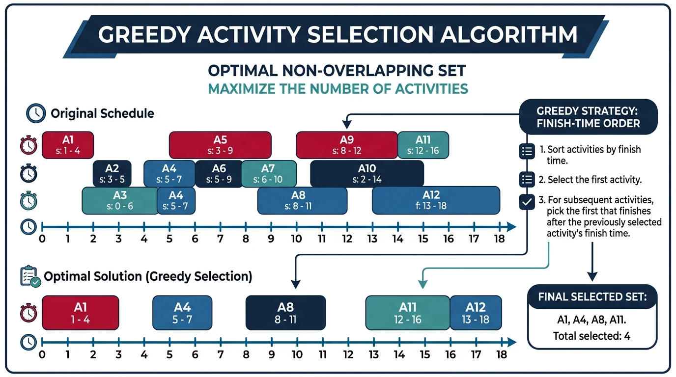
Activity Selection

Given a set of activities with start and end times, select the maximum number of non-overlapping activities. The greedy strategy is deceptively simple: sort by end time, then always pick the activity that finishes earliest and doesn't overlap with the last selected. This works because finishing early leaves the most room for future activities — a provably optimal greedy choice. Time: \(O(n \log n)\) for sorting.

def activity_selection(activities):
    """
    Select maximum non-overlapping activities
    activities: list of (start, end) tuples
    Time: O(n log n), Space: O(1)
    """
    # Sort by end time
    activities = sorted(activities, key=lambda x: x[1])
    
    selected = [activities[0]]
    last_end = activities[0][1]
    
    for start, end in activities[1:]:
        if start >= last_end:  # Non-overlapping
            selected.append((start, end))
            last_end = end
    
    return selected

# Example
activities = [(1, 4), (3, 5), (0, 6), (5, 7), (3, 9), (5, 9), (6, 10), (8, 11), (8, 12), (2, 14), (12, 16)]
result = activity_selection(activities)
print(f"Activities: {len(activities)}")
print(f"Max selected: {len(result)}")
print(f"Selected: {result}")

// Activity Selection - Maximum non-overlapping activities
// Time: O(n log n), Space: O(1)
#include <vector>
#include <algorithm>

class ActivitySelection {
public:
    static std::vector<std::pair<int, int>> select(
            std::vector<std::pair<int, int>>& activities) {
        // Sort by end time
        std::sort(activities.begin(), activities.end(),
                  [](auto& a, auto& b) { return a.second < b.second; });
        
        std::vector<std::pair<int, int>> selected;
        selected.push_back(activities[0]);
        int lastEnd = activities[0].second;
        
        for (int i = 1; i < activities.size(); i++) {
            if (activities[i].first >= lastEnd) {
                selected.push_back(activities[i]);
                lastEnd = activities[i].second;
            }
        }
        return selected;
    }
};

// Activity Selection - Maximum non-overlapping activities
// Time: O(n log n), Space: O(1)
import java.util.*;

class ActivitySelection {
    public static List<int[]> select(int[][] activities) {
        // Sort by end time
        Arrays.sort(activities, (a, b) -> a[1] - b[1]);
        
        List<int[]> selected = new ArrayList<>();
        selected.add(activities[0]);
        int lastEnd = activities[0][1];
        
        for (int i = 1; i < activities.length; i++) {
            if (activities[i][0] >= lastEnd) {
                selected.add(activities[i]);
                lastEnd = activities[i][1];
            }
        }
        return selected;
    }
}

Jump Game

Given an array where each element represents the maximum jump length from that position, determine (a) if you can reach the last index, and (b) the minimum number of jumps. The greedy insight: maintain the farthest reachable index as you scan left-to-right. If your current position ever exceeds the farthest reach, you're stuck. For minimum jumps, use a "BFS-like" greedy: track the current reachable range (a "level"), and when you exhaust it, jump to the new farthest point.

def can_jump(nums):
    """
    LeetCode 55: Jump Game
    Can you reach the last index?
    Time: O(n), Space: O(1)
    """
    max_reach = 0
    
    for i, jump in enumerate(nums):
        if i > max_reach:
            return False
        max_reach = max(max_reach, i + jump)
    
    return True

def min_jumps(nums):
    """
    LeetCode 45: Jump Game II
    Minimum jumps to reach end
    Time: O(n), Space: O(1)
    """
    if len(nums) <= 1:
        return 0
    
    jumps = 0
    current_end = 0
    farthest = 0
    
    for i in range(len(nums) - 1):
        farthest = max(farthest, i + nums[i])
        
        if i == current_end:
            jumps += 1
            current_end = farthest
            
            if current_end >= len(nums) - 1:
                break
    
    return jumps

# Examples
nums1 = [2, 3, 1, 1, 4]
print(f"Array: {nums1}")
print(f"Can reach end: {can_jump(nums1)}")  # True
print(f"Min jumps: {min_jumps(nums1)}")  # 2

nums2 = [3, 2, 1, 0, 4]
print(f"\nArray: {nums2}")
print(f"Can reach end: {can_jump(nums2)}")  # False

// LeetCode 55: Jump Game & LeetCode 45: Jump Game II
#include <vector>
#include <algorithm>

class JumpGame {
public:
    // Can reach the last index?
    static bool canJump(std::vector<int>& nums) {
        int maxReach = 0;
        for (int i = 0; i < nums.size(); i++) {
            if (i > maxReach) return false;
            maxReach = std::max(maxReach, i + nums[i]);
        }
        return true;
    }
    
    // Minimum jumps to reach end
    static int minJumps(std::vector<int>& nums) {
        if (nums.size() <= 1) return 0;
        
        int jumps = 0, currentEnd = 0, farthest = 0;
        for (int i = 0; i < nums.size() - 1; i++) {
            farthest = std::max(farthest, i + nums[i]);
            if (i == currentEnd) {
                jumps++;
                currentEnd = farthest;
                if (currentEnd >= nums.size() - 1) break;
            }
        }
        return jumps;
    }
};

// LeetCode 55: Jump Game & LeetCode 45: Jump Game II

class JumpGame {
    // Can reach the last index?
    public static boolean canJump(int[] nums) {
        int maxReach = 0;
        for (int i = 0; i < nums.length; i++) {
            if (i > maxReach) return false;
            maxReach = Math.max(maxReach, i + nums[i]);
        }
        return true;
    }
    
    // Minimum jumps to reach end
    public static int minJumps(int[] nums) {
        if (nums.length <= 1) return 0;
        
        int jumps = 0, currentEnd = 0, farthest = 0;
        for (int i = 0; i < nums.length - 1; i++) {
            farthest = Math.max(farthest, i + nums[i]);
            if (i == currentEnd) {
                jumps++;
                currentEnd = farthest;
                if (currentEnd >= nums.length - 1) break;
            }
        }
        return jumps;
    }
}

Interval Scheduling

A family of problems involving overlapping intervals: merge overlapping intervals, find minimum meeting rooms, or insert a new interval. The common preprocessing step is sorting by start time (or end time, depending on the variant). For merging: sort by start, then extend the current interval's end if the next overlaps; otherwise close and start a new interval. For meeting rooms: count the maximum overlap at any point (equivalent to a sweep line or min-heap approach).

def erase_overlap_intervals(intervals):
    """
    LeetCode 435: Non-overlapping Intervals
    Minimum intervals to remove for no overlap
    Time: O(n log n), Space: O(1)
    """
    if not intervals:
        return 0
    
    # Sort by end time
    intervals.sort(key=lambda x: x[1])
    
    removals = 0
    prev_end = intervals[0][1]
    
    for i in range(1, len(intervals)):
        if intervals[i][0] < prev_end:  # Overlap
            removals += 1
        else:
            prev_end = intervals[i][1]
    
    return removals

def merge_intervals(intervals):
    """
    LeetCode 56: Merge Intervals
    Time: O(n log n), Space: O(n)
    """
    if not intervals:
        return []
    
    # Sort by start time
    intervals.sort(key=lambda x: x[0])
    
    merged = [intervals[0]]
    
    for start, end in intervals[1:]:
        if start <= merged[-1][1]:  # Overlap
            merged[-1][1] = max(merged[-1][1], end)
        else:
            merged.append([start, end])
    
    return merged

# Examples
intervals1 = [[1, 2], [2, 3], [3, 4], [1, 3]]
print(f"Intervals: {intervals1}")
print(f"Remove to eliminate overlap: {erase_overlap_intervals(intervals1)}")  # 1

intervals2 = [[1, 3], [2, 6], [8, 10], [15, 18]]
print(f"\nIntervals: {intervals2}")
print(f"Merged: {merge_intervals(intervals2)}")  # [[1,6],[8,10],[15,18]]

// LeetCode 435: Non-overlapping Intervals
// LeetCode 56: Merge Intervals
#include <vector>
#include <algorithm>

class IntervalScheduling {
public:
    // Min removals for no overlap
    static int eraseOverlapIntervals(std::vector<std::vector<int>>& intervals) {
        if (intervals.empty()) return 0;
        
        std::sort(intervals.begin(), intervals.end(),
                  [](auto& a, auto& b) { return a[1] < b[1]; });
        
        int removals = 0, prevEnd = intervals[0][1];
        for (int i = 1; i < intervals.size(); i++) {
            if (intervals[i][0] < prevEnd)
                removals++;
            else
                prevEnd = intervals[i][1];
        }
        return removals;
    }
    
    // Merge overlapping intervals
    static std::vector<std::vector<int>> mergeIntervals(
            std::vector<std::vector<int>>& intervals) {
        if (intervals.empty()) return {};
        
        std::sort(intervals.begin(), intervals.end());
        std::vector<std::vector<int>> merged = {intervals[0]};
        
        for (int i = 1; i < intervals.size(); i++) {
            if (intervals[i][0] <= merged.back()[1])
                merged.back()[1] = std::max(merged.back()[1], intervals[i][1]);
            else
                merged.push_back(intervals[i]);
        }
        return merged;
    }
};

// LeetCode 435: Non-overlapping Intervals
// LeetCode 56: Merge Intervals
import java.util.*;

class IntervalScheduling {
    // Min removals for no overlap
    public static int eraseOverlapIntervals(int[][] intervals) {
        if (intervals.length == 0) return 0;
        
        Arrays.sort(intervals, (a, b) -> a[1] - b[1]);
        
        int removals = 0, prevEnd = intervals[0][1];
        for (int i = 1; i < intervals.length; i++) {
            if (intervals[i][0] < prevEnd)
                removals++;
            else
                prevEnd = intervals[i][1];
        }
        return removals;
    }
    
    // Merge overlapping intervals
    public static int[][] mergeIntervals(int[][] intervals) {
        if (intervals.length == 0) return new int[][]{};
        
        Arrays.sort(intervals, (a, b) -> a[0] - b[0]);
        List<int[]> merged = new ArrayList<>();
        merged.add(intervals[0]);
        
        for (int i = 1; i < intervals.length; i++) {
            int[] last = merged.get(merged.size() - 1);
            if (intervals[i][0] <= last[1])
                last[1] = Math.max(last[1], intervals[i][1]);
            else
                merged.add(intervals[i]);
        }
        return merged.toArray(new int[merged.size()][]);
    }
}

Backtracking

Backtracking is a systematic way to explore all possible solutions by building candidates incrementally and abandoning ("backtracking") candidates that fail to satisfy constraints.

Backtracking Template

def backtrack(candidate):
    if is_solution(candidate):
        output(candidate)
        return
    
    for choice in choices:
        if is_valid(choice):
            make_choice(choice)
            backtrack(candidate)
            undo_choice(choice)  # Backtrack

Permutations

Generate all possible orderings of a given set. At each position, try every unused element, recurse to fill the next position, then undo the choice (backtrack). The decision tree has \(n!\) leaves (one per permutation). Key constraint: use a "used" boolean array to avoid placing the same element twice. For duplicates, sort first and skip adjacent identical unused elements to avoid duplicate permutations.

def permute(nums):
    """
    LeetCode 46: Permutations
    Generate all permutations
    Time: O(n! * n), Space: O(n)
    """
    result = []
    
    def backtrack(current, remaining):
        if not remaining:
            result.append(current[:])
            return
        
        for i in range(len(remaining)):
            # Make choice
            current.append(remaining[i])
            
            # Recurse with remaining elements
            backtrack(current, remaining[:i] + remaining[i+1:])
            
            # Undo choice
            current.pop()
    
    backtrack([], nums)
    return result

# Example
nums = [1, 2, 3]
print(f"Permutations of {nums}:")
for perm in permute(nums):
    print(f"  {perm}")

// LeetCode 46: Permutations
// Time: O(n! * n), Space: O(n)
#include <vector>

class Permutations {
public:
    static std::vector<std::vector<int>> permute(std::vector<int>& nums) {
        std::vector<std::vector<int>> result;
        std::vector<int> current;
        std::vector<bool> used(nums.size(), false);
        backtrack(nums, current, used, result);
        return result;
    }
    
private:
    static void backtrack(std::vector<int>& nums, std::vector<int>& current,
                          std::vector<bool>& used, std::vector<std::vector<int>>& result) {
        if (current.size() == nums.size()) {
            result.push_back(current);
            return;
        }
        
        for (int i = 0; i < nums.size(); i++) {
            if (used[i]) continue;
            
            current.push_back(nums[i]);
            used[i] = true;
            backtrack(nums, current, used, result);
            current.pop_back();
            used[i] = false;
        }
    }
};

// LeetCode 46: Permutations
// Time: O(n! * n), Space: O(n)
import java.util.*;

class Permutations {
    public static List<List<Integer>> permute(int[] nums) {
        List<List<Integer>> result = new ArrayList<>();
        backtrack(nums, new ArrayList<>(), new boolean[nums.length], result);
        return result;
    }
    
    private static void backtrack(int[] nums, List<Integer> current,
                                   boolean[] used, List<List<Integer>> result) {
        if (current.size() == nums.length) {
            result.add(new ArrayList<>(current));
            return;
        }
        
        for (int i = 0; i < nums.length; i++) {
            if (used[i]) continue;
            
            current.add(nums[i]);
            used[i] = true;
            backtrack(nums, current, used, result);
            current.remove(current.size() - 1);
            used[i] = false;
        }
    }
}

Subsets

Generate all \(2^n\) subsets (the power set) of a given array. At each element, make a binary choice: include it or exclude it. The recursion tree branches two ways at each level, giving \(2^n\) total subsets. Implementation uses an index \(i\) to avoid revisiting earlier elements (since subset order doesn't matter). This is the foundation for many search problems — Subsets II (with duplicates) adds a skip condition for consecutive identical values.

def subsets(nums):
    """
    LeetCode 78: Subsets
    Generate all subsets (power set)
    Time: O(2^n * n), Space: O(n)
    """
    result = []
    
    def backtrack(start, current):
        result.append(current[:])
        
        for i in range(start, len(nums)):
            current.append(nums[i])
            backtrack(i + 1, current)
            current.pop()
    
    backtrack(0, [])
    return result

def subsets_with_dup(nums):
    """
    LeetCode 90: Subsets II (with duplicates)
    """
    result = []
    nums.sort()
    
    def backtrack(start, current):
        result.append(current[:])
        
        for i in range(start, len(nums)):
            # Skip duplicates
            if i > start and nums[i] == nums[i-1]:
                continue
            current.append(nums[i])
            backtrack(i + 1, current)
            current.pop()
    
    backtrack(0, [])
    return result

# Example
nums = [1, 2, 3]
print(f"Subsets of {nums}:")
for subset in subsets(nums):
    print(f"  {subset}")

// LeetCode 78: Subsets & LeetCode 90: Subsets II
// Time: O(2^n * n), Space: O(n)
#include <vector>
#include <algorithm>

class Subsets {
public:
    static std::vector<std::vector<int>> subsets(std::vector<int>& nums) {
        std::vector<std::vector<int>> result;
        std::vector<int> current;
        backtrack(nums, 0, current, result);
        return result;
    }
    
    // With duplicates
    static std::vector<std::vector<int>> subsetsWithDup(std::vector<int>& nums) {
        std::sort(nums.begin(), nums.end());
        std::vector<std::vector<int>> result;
        std::vector<int> current;
        backtrackWithDup(nums, 0, current, result);
        return result;
    }
    
private:
    static void backtrack(std::vector<int>& nums, int start,
                          std::vector<int>& current, std::vector<std::vector<int>>& result) {
        result.push_back(current);
        for (int i = start; i < nums.size(); i++) {
            current.push_back(nums[i]);
            backtrack(nums, i + 1, current, result);
            current.pop_back();
        }
    }
    
    static void backtrackWithDup(std::vector<int>& nums, int start,
                                  std::vector<int>& current, std::vector<std::vector<int>>& result) {
        result.push_back(current);
        for (int i = start; i < nums.size(); i++) {
            if (i > start && nums[i] == nums[i-1]) continue;  // Skip dups
            current.push_back(nums[i]);
            backtrackWithDup(nums, i + 1, current, result);
            current.pop_back();
        }
    }
};

// LeetCode 78: Subsets & LeetCode 90: Subsets II
import java.util.*;

class Subsets {
    public static List<List<Integer>> subsets(int[] nums) {
        List<List<Integer>> result = new ArrayList<>();
        backtrack(nums, 0, new ArrayList<>(), result);
        return result;
    }
    
    // With duplicates
    public static List<List<Integer>> subsetsWithDup(int[] nums) {
        Arrays.sort(nums);
        List<List<Integer>> result = new ArrayList<>();
        backtrackWithDup(nums, 0, new ArrayList<>(), result);
        return result;
    }
    
    private static void backtrack(int[] nums, int start,
                                   List<Integer> current, List<List<Integer>> result) {
        result.add(new ArrayList<>(current));
        for (int i = start; i < nums.length; i++) {
            current.add(nums[i]);
            backtrack(nums, i + 1, current, result);
            current.remove(current.size() - 1);
        }
    }
    
    private static void backtrackWithDup(int[] nums, int start,
                                          List<Integer> current, List<List<Integer>> result) {
        result.add(new ArrayList<>(current));
        for (int i = start; i < nums.length; i++) {
            if (i > start && nums[i] == nums[i-1]) continue;  // Skip dups
            current.add(nums[i]);
            backtrackWithDup(nums, i + 1, current, result);
            current.remove(current.size() - 1);
        }
    }
}

Combination Sum

Find all unique combinations that sum to a target. Unlike subsets (which enumerate all), here we prune branches where the running sum exceeds the target — this is backtracking's power over brute force. The key decision at each step: which candidate to add next (starting from index \(i\) to avoid reusing earlier positions). In the "reuse allowed" variant, recurse with the same index \(i\) (not \(i+1\)); in "use once" variants, advance to \(i+1\).

def combination_sum(candidates, target):
    """
    LeetCode 39: Combination Sum
    Find combinations that sum to target (can reuse)
    Time: O(2^target), Space: O(target)
    """
    result = []
    
    def backtrack(start, current, remaining):
        if remaining == 0:
            result.append(current[:])
            return
        
        if remaining < 0:
            return
        
        for i in range(start, len(candidates)):
            current.append(candidates[i])
            # Can reuse same element, so pass i (not i+1)
            backtrack(i, current, remaining - candidates[i])
            current.pop()
    
    backtrack(0, [], target)
    return result

# Example
candidates = [2, 3, 6, 7]
target = 7
print(f"Candidates: {candidates}, Target: {target}")
print(f"Combinations:")
for combo in combination_sum(candidates, target):
    print(f"  {combo}")

// LeetCode 39: Combination Sum
// Time: O(2^target), Space: O(target)
#include <vector>

class CombinationSum {
public:
    static std::vector<std::vector<int>> combinationSum(
            std::vector<int>& candidates, int target) {
        std::vector<std::vector<int>> result;
        std::vector<int> current;
        backtrack(candidates, target, 0, current, result);
        return result;
    }
    
private:
    static void backtrack(std::vector<int>& candidates, int remaining, int start,
                          std::vector<int>& current, std::vector<std::vector<int>>& result) {
        if (remaining == 0) {
            result.push_back(current);
            return;
        }
        if (remaining < 0) return;
        
        for (int i = start; i < candidates.size(); i++) {
            current.push_back(candidates[i]);
            backtrack(candidates, remaining - candidates[i], i, current, result);  // i, not i+1
            current.pop_back();
        }
    }
};

// LeetCode 39: Combination Sum
// Time: O(2^target), Space: O(target)
import java.util.*;

class CombinationSum {
    public static List<List<Integer>> combinationSum(int[] candidates, int target) {
        List<List<Integer>> result = new ArrayList<>();
        backtrack(candidates, target, 0, new ArrayList<>(), result);
        return result;
    }
    
    private static void backtrack(int[] candidates, int remaining, int start,
                                   List<Integer> current, List<List<Integer>> result) {
        if (remaining == 0) {
            result.add(new ArrayList<>(current));
            return;
        }
        if (remaining < 0) return;
        
        for (int i = start; i < candidates.length; i++) {
            current.add(candidates[i]);
            backtrack(candidates, remaining - candidates[i], i, current, result);  // i, not i+1
            current.remove(current.size() - 1);
        }
    }
}

N-Queens

Place \(N\) queens on an \(N \times N\) chessboard so no two queens attack each other (no shared row, column, or diagonal). This is the classic constraint-satisfaction backtracking problem. Place queens row by row; for each row, try each column and check if it's safe (no queen in the same column, or either diagonal). Use sets or boolean arrays to track occupied columns and diagonals. The diagonal trick: cells on the same diagonal have equal \(row - col\) (main) or \(row + col\) (anti-diagonal).

def solve_n_queens(n):
    """
    LeetCode 51: N-Queens
    Place n queens on n×n board with no attacks
    Time: O(n!), Space: O(n)
    """
    result = []
    board = [['.'] * n for _ in range(n)]
    
    # Track columns and diagonals under attack
    cols = set()
    diag1 = set()  # row - col
    diag2 = set()  # row + col
    
    def backtrack(row):
        if row == n:
            result.append([''.join(row) for row in board])
            return
        
        for col in range(n):
            if col in cols or (row - col) in diag1 or (row + col) in diag2:
                continue
            
            # Place queen
            board[row][col] = 'Q'
            cols.add(col)
            diag1.add(row - col)
            diag2.add(row + col)
            
            backtrack(row + 1)
            
            # Remove queen
            board[row][col] = '.'
            cols.remove(col)
            diag1.remove(row - col)
            diag2.remove(row + col)
    
    backtrack(0)
    return result

# Example
n = 4
solutions = solve_n_queens(n)
print(f"{n}-Queens has {len(solutions)} solutions:")
for i, sol in enumerate(solutions):
    print(f"\nSolution {i+1}:")
    for row in sol:
        print(f"  {row}")

// LeetCode 51: N-Queens
// Time: O(n!), Space: O(n)
#include <vector>
#include <string>
#include <unordered_set>

class NQueens {
public:
    static std::vector<std::vector<std::string>> solveNQueens(int n) {
        std::vector<std::vector<std::string>> result;
        std::vector<std::string> board(n, std::string(n, '.'));
        std::unordered_set<int> cols, diag1, diag2;
        backtrack(n, 0, board, cols, diag1, diag2, result);
        return result;
    }
    
private:
    static void backtrack(int n, int row, std::vector<std::string>& board,
                          std::unordered_set<int>& cols,
                          std::unordered_set<int>& diag1,
                          std::unordered_set<int>& diag2,
                          std::vector<std::vector<std::string>>& result) {
        if (row == n) {
            result.push_back(board);
            return;
        }
        
        for (int col = 0; col < n; col++) {
            if (cols.count(col) || diag1.count(row - col) || diag2.count(row + col))
                continue;
            
            board[row][col] = 'Q';
            cols.insert(col);
            diag1.insert(row - col);
            diag2.insert(row + col);
            
            backtrack(n, row + 1, board, cols, diag1, diag2, result);
            
            board[row][col] = '.';
            cols.erase(col);
            diag1.erase(row - col);
            diag2.erase(row + col);
        }
    }
};

// LeetCode 51: N-Queens
// Time: O(n!), Space: O(n)
import java.util.*;

class NQueens {
    public static List<List<String>> solveNQueens(int n) {
        List<List<String>> result = new ArrayList<>();
        char[][] board = new char[n][n];
        for (char[] row : board) Arrays.fill(row, '.');
        Set<Integer> cols = new HashSet<>();
        Set<Integer> diag1 = new HashSet<>();
        Set<Integer> diag2 = new HashSet<>();
        backtrack(n, 0, board, cols, diag1, diag2, result);
        return result;
    }
    
    private static void backtrack(int n, int row, char[][] board,
                                   Set<Integer> cols, Set<Integer> diag1, Set<Integer> diag2,
                                   List<List<String>> result) {
        if (row == n) {
            List<String> solution = new ArrayList<>();
            for (char[] r : board) solution.add(new String(r));
            result.add(solution);
            return;
        }
        
        for (int col = 0; col < n; col++) {
            if (cols.contains(col) || diag1.contains(row - col) || diag2.contains(row + col))
                continue;
            
            board[row][col] = 'Q';
            cols.add(col);
            diag1.add(row - col);
            diag2.add(row + col);
            
            backtrack(n, row + 1, board, cols, diag1, diag2, result);
            
            board[row][col] = '.';
            cols.remove(col);
            diag1.remove(row - col);
            diag2.remove(row + col);
        }
    }
}

LeetCode Practice Problems

Essential Problems

#	Problem	Difficulty	Key Concept
200	Number of Islands	Medium	Graph DFS/BFS
207	Course Schedule	Medium	Topological Sort
743	Network Delay Time	Medium	Dijkstra
70	Climbing Stairs	Easy	1D DP
198	House Robber	Medium	1D DP
322	Coin Change	Medium	DP - Unbounded Knapsack
1143	Longest Common Subsequence	Medium	2D DP
55	Jump Game	Medium	Greedy
46	Permutations	Medium	Backtracking
51	N-Queens	Hard	Backtracking

Complete DSA Series

FAANG Interview Preparation - Series Complete! ??

Stack & Applications
Queue & Variants
Trees & Traversals
BST & Balanced Trees
Heaps, Sorting & Hashing
Graphs, DP, Greedy & Backtracking (You are here)

Congratulations! You've completed the entire 12-part DSA series. Practice these concepts consistently on LeetCode, and you'll be well-prepared for FAANG interviews!

Quick Check — Test Yourself

Given graph: A-B, A-C, B-D, C-D, D-E. Find the shortest path A→E using Dijkstra. Show the priority queue state at each step.
Define “optimal substructure” and “overlapping subproblems”. Give one problem that has both, one that has only optimal substructure.
Solve coin change for coins=[1,5,11] and amount=15. Is greedy optimal here? Why or why not?

Common Bugs

Not settling nodes in Dijkstra: When popping, check if dist > distances[node]: continue. Without this, stale heap entries cause wrong results.
DP array size off by one: For coin change up to amount n, allocate dp[n+1]. Missing the +1 causes an out-of-bounds on the target value.
Confusing greedy with DP: Greedy works when local optimal = global optimal. Non-canonical coin systems break greedy but DP handles them correctly.

Interview Lens

For graph problems, always clarify: directed or undirected? Weighted? Can it have cycles? Negative weights? Each combination unlocks a different algorithm. For DP: define dp[i] meaning precisely, write the recurrence, handle base cases, then decide top-down vs bottom-up.

Production Lens

Google Maps uses A* (Dijkstra + heuristic). Social networks use BFS for degree-of-separation. Backtracking powers SAT solvers and scheduling. DP appears in bioinformatics (sequence alignment), financial option pricing (binomial models), and compiler optimisation (instruction selection).

Table of Contents