Complete DSA Series Part 1: Foundations, Memory & Complexity

FAANG Interview Prep

Your 12-step learning path • Currently on Step 1

Foundations, Memory & Complexity

Big-O notation, time/space analysis, memory layout

You Are Here

Introduction: Why DSA Matters

Data Structures and Algorithms (DSA) form the core foundation of computer science and software engineering. Whether you're preparing for FAANG interviews, building scalable systems, or solving complex problems, mastering DSA is essential.

DSA Learning Roadmap

flowchart TD
    A["1. Foundations
Big-O • Memory Layout
Time & Space Analysis"] --> B["2. Recursion
Call Stack • Memoization
Divide & Conquer"]
    B --> C["3. Arrays
Static & Dynamic
Two Pointers • Sliding Window"]
    C --> D["4. Strings
Pattern Matching
KMP • Rabin-Karp"]
    C --> E["5. Matrices
2D Arrays • Sparse
Traversal Patterns"]
    D --> F["6. Linked Lists
Singly • Doubly • Circular
Fast/Slow Pointers"]
    E --> F
    F --> G["7. Stacks
LIFO • Expression Eval
Monotonic Stack"]
    F --> H["8. Queues
FIFO • Deque
Priority Queue"]
    G --> I["9. Trees
Binary Trees • Traversals
Expression Trees"]
    H --> I
    I --> J["10. BST & Balanced
AVL • Red-Black
B-Trees"]
    J --> K["11. Heaps & Hashing
Min/Max Heap • Heapsort
Hash Tables"]
    K --> L["12. Graphs & DP
BFS • DFS • Shortest Path
Dynamic Programming"]

    style A fill:#3B9797,stroke:#132440,color:#fff
    style B fill:#3B9797,stroke:#132440,color:#fff
    style C fill:#16476A,stroke:#132440,color:#fff
    style D fill:#16476A,stroke:#132440,color:#fff
    style E fill:#16476A,stroke:#132440,color:#fff
    style F fill:#16476A,stroke:#132440,color:#fff
    style G fill:#132440,stroke:#3B9797,color:#fff
    style H fill:#132440,stroke:#3B9797,color:#fff
    style I fill:#132440,stroke:#3B9797,color:#fff
    style J fill:#BF092F,stroke:#132440,color:#fff
    style K fill:#BF092F,stroke:#132440,color:#fff
    style L fill:#BF092F,stroke:#132440,color:#fff

                            
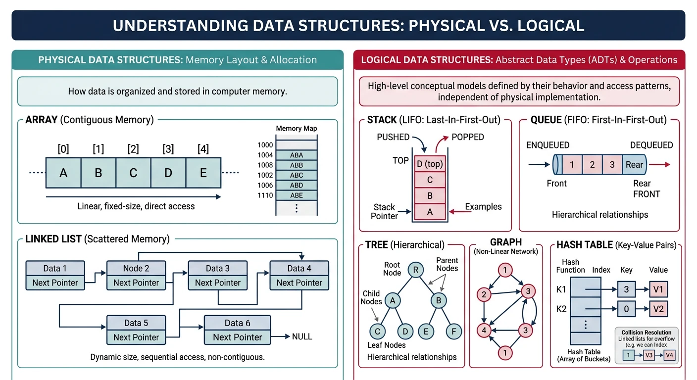
                            Key Insight: DSA isn't just about passing interviews—it's about writing efficient code that scales. Understanding how data is organized and manipulated determines whether your solution handles 100 users or 100 million.
                        

Physical vs Logical Data Structures

Data structures can be classified based on how they are stored in memory (physical) and how they behave logically.

Diagram showing physical data structures (arrays and linked lists) versus logical data structures (stacks, queues, trees, graphs, hash tables) — Physical vs Logical Data Structures — physical structures define memory layout while logical structures define behavior and operations

Data Structure Taxonomy

graph TD
    DS["Data Structures"]
    DS --> Linear["Linear"]
    DS --> NonLinear["Non-Linear"]

    Linear --> Arr["Array"]
    Linear --> LL["Linked List"]
    Linear --> Stack["Stack"]
    Linear --> Queue["Queue"]

    NonLinear --> Tree["Tree"]
    NonLinear --> Graph["Graph"]
    NonLinear --> Hash["Hash Table"]

    style DS fill:#132440,stroke:#132440,color:#fff
    style Linear fill:#16476A,stroke:#132440,color:#fff
    style NonLinear fill:#3B9797,stroke:#132440,color:#fff

Physical Data Structures

What are Data Structures?

A data structure is a specialized format for organizing, processing, retrieving, and storing data. Think of it like organizing items in a warehouse—different organization methods work better for different purposes.

Why learn this? The right data structure can make the difference between an algorithm that runs in milliseconds vs. one that takes hours!

Physical Data Structures

Physical structures define how data is actually stored in memory:

Arrays - Contiguous memory allocation, fixed size at creation. Elements stored one after another in memory.
Linked Lists - Non-contiguous nodes connected via pointers/references, dynamic size. Each node stores data + address of next node.

Logical Data Structures

Logical structures define the behavior and operations, implemented using physical structures:

Linear: Stack (LIFO - Last In First Out), Queue (FIFO - First In First Out), Deque (Double-ended Queue)
Non-Linear: Trees (hierarchical), Graphs (interconnected nodes)
Tabular: Hash Tables (key-value mapping)

Key Insight

A Stack can be implemented using an Array OR a Linked List. The physical structure is the "how", while the logical structure is the "what behavior".

# Physical vs Logical Data Structures in Python
import array
from collections import deque

# PHYSICAL: Array - contiguous memory
arr = array.array('i', [1, 2, 3, 4, 5])
print(f"Array: {list(arr)}")

# PHYSICAL: Linked List concept
class Node:
    def __init__(self, data):
        self.data = data
        self.next = None

head = Node(10)
head.next = Node(20)
head.next.next = Node(30)

# Traverse linked list
current = head
print("Linked List: ", end="")
while current:
    print(current.data, end=" -> " if current.next else "\n")
    current = current.next

# LOGICAL: Stack (LIFO) - can use list or linked list underneath
stack = []
stack.append(10)  # push
stack.append(20)  # push
print(f"Stack pop: {stack.pop()}")  # Output: 20

# LOGICAL: Queue (FIFO) - using deque for O(1) operations
queue = deque()
queue.append(10)   # enqueue
queue.append(20)   # enqueue
print(f"Queue dequeue: {queue.popleft()}")  # Output: 10

// Physical vs Logical Data Structures in C++
#include <iostream>
#include <stack>
#include <queue>
using namespace std;

// PHYSICAL: Linked List Node
struct Node {
    int data;
    Node* next;
    Node(int val) : data(val), next(nullptr) {}
};

int main() {
    // PHYSICAL: Array - contiguous memory
    int arr[5] = {1, 2, 3, 4, 5};
    cout << "Array: ";
    for (int i = 0; i < 5; i++) {
        cout << arr[i] << " ";
    }
    cout << endl;
    
    // PHYSICAL: Linked List
    Node* head = new Node(10);
    head->next = new Node(20);
    head->next->next = new Node(30);
    
    cout << "Linked List: ";
    Node* current = head;
    while (current) {
        cout << current->data;
        if (current->next) cout << " -> ";
        current = current->next;
    }
    cout << endl;
    
    // LOGICAL: Stack (LIFO) using STL
    stack<int> s;
    s.push(10);
    s.push(20);
    cout << "Stack pop: " << s.top() << endl;  // 20
    s.pop();
    
    // LOGICAL: Queue (FIFO) using STL
    queue<int> q;
    q.push(10);
    q.push(20);
    cout << "Queue dequeue: " << q.front() << endl;  // 10
    q.pop();
    
    // Cleanup
    while (head) {
        Node* temp = head;
        head = head->next;
        delete temp;
    }
    
    return 0;
}

// Physical vs Logical Data Structures in Java
import java.util.*;

public class DataStructuresDemo {
    // PHYSICAL: Linked List Node
    static class Node {
        int data;
        Node next;
        Node(int data) { this.data = data; }
    }
    
    public static void main(String[] args) {
        // PHYSICAL: Array - contiguous memory
        int[] arr = {1, 2, 3, 4, 5};
        System.out.print("Array: ");
        for (int num : arr) {
            System.out.print(num + " ");
        }
        System.out.println();
        
        // PHYSICAL: Linked List
        Node head = new Node(10);
        head.next = new Node(20);
        head.next.next = new Node(30);
        
        System.out.print("Linked List: ");
        Node current = head;
        while (current != null) {
            System.out.print(current.data);
            if (current.next != null) System.out.print(" -> ");
            current = current.next;
        }
        System.out.println();
        
        // LOGICAL: Stack (LIFO)
        Stack<Integer> stack = new Stack<>();
        stack.push(10);
        stack.push(20);
        System.out.println("Stack pop: " + stack.pop());  // 20
        
        // LOGICAL: Queue (FIFO)
        Queue<Integer> queue = new LinkedList<>();
        queue.offer(10);
        queue.offer(20);
        System.out.println("Queue dequeue: " + queue.poll());  // 10
    }
}

Abstract Data Types (ADT)

What is an ADT?

An Abstract Data Type (ADT) defines what operations can be performed, not how they're implemented. It's like a contract or interface that specifies behavior without implementation details.

Real-world analogy: A TV remote is an ADT—you know pressing "Volume Up" increases volume, but you don't need to know the internal circuitry!

List ADT Operations

insert(index, element) - Insert element at position
delete(index) - Remove element at position
get(index) - Retrieve element at position
set(index, element) - Update element at position
length() - Return number of elements
search(element) - Find element position

Implementations: Can use Array-based (fast access), Linked List-based (fast insert/delete), or Dynamic Array (balanced)

# List ADT Implementation in Python
from abc import ABC, abstractmethod

# Define the ADT interface
class ListADT(ABC):
    @abstractmethod
    def insert(self, index, element): pass
    
    @abstractmethod
    def delete(self, index): pass
    
    @abstractmethod
    def get(self, index): pass
    
    @abstractmethod
    def set(self, index, element): pass
    
    @abstractmethod
    def length(self): pass
    
    @abstractmethod
    def search(self, element): pass

# Array-based implementation
class ArrayList(ListADT):
    def __init__(self, capacity=10):
        self.data = [None] * capacity
        self.size = 0
        self.capacity = capacity
    
    def insert(self, index, element):
        if self.size >= self.capacity:
            raise RuntimeError("Array is full")
        # Shift elements right
        for i in range(self.size, index, -1):
            self.data[i] = self.data[i - 1]
        self.data[index] = element
        self.size += 1
    
    def delete(self, index):
        if index >= self.size:
            raise IndexError("Index out of bounds")
        element = self.data[index]
        # Shift elements left
        for i in range(index, self.size - 1):
            self.data[i] = self.data[i + 1]
        self.size -= 1
        return element
    
    def get(self, index):
        if index >= self.size:
            raise IndexError("Index out of bounds")
        return self.data[index]
    
    def set(self, index, element):
        if index >= self.size:
            raise IndexError("Index out of bounds")
        self.data[index] = element
    
    def length(self):
        return self.size
    
    def search(self, element):
        for i in range(self.size):
            if self.data[i] == element:
                return i
        return -1

# Test
arr_list = ArrayList(10)
arr_list.insert(0, 10)
arr_list.insert(1, 20)
arr_list.insert(1, 15)  # Insert in middle
print(f"Length: {arr_list.length()}")  # 3
print(f"Element at 1: {arr_list.get(1)}")  # 15
print(f"Search 20: index {arr_list.search(20)}")  # 2

// List ADT Implementation in C++
#include <iostream>
#include <stdexcept>
using namespace std;

// Abstract base class (interface)
template<typename T>
class ListADT {
public:
    virtual void insert(int index, T element) = 0;
    virtual T remove(int index) = 0;
    virtual T get(int index) = 0;
    virtual void set(int index, T element) = 0;
    virtual int length() = 0;
    virtual int search(T element) = 0;
    virtual ~ListADT() {}
};

// Array-based implementation
template<typename T>
class ArrayList : public ListADT<T> {
private:
    T* data;
    int size;
    int capacity;

public:
    ArrayList(int cap = 10) : capacity(cap), size(0) {
        data = new T[capacity];
    }
    
    ~ArrayList() { delete[] data; }
    
    void insert(int index, T element) override {
        if (size >= capacity) 
            throw runtime_error("Array is full");
        // Shift elements right
        for (int i = size; i > index; i--) {
            data[i] = data[i - 1];
        }
        data[index] = element;
        size++;
    }
    
    T remove(int index) override {
        if (index >= size) 
            throw out_of_range("Index out of bounds");
        T element = data[index];
        // Shift elements left
        for (int i = index; i < size - 1; i++) {
            data[i] = data[i + 1];
        }
        size--;
        return element;
    }
    
    T get(int index) override {
        if (index >= size)
            throw out_of_range("Index out of bounds");
        return data[index];
    }
    
    void set(int index, T element) override {
        if (index >= size)
            throw out_of_range("Index out of bounds");
        data[index] = element;
    }
    
    int length() override { return size; }
    
    int search(T element) override {
        for (int i = 0; i < size; i++) {
            if (data[i] == element) return i;
        }
        return -1;
    }
};

int main() {
    ArrayList<int> arrList(10);
    arrList.insert(0, 10);
    arrList.insert(1, 20);
    arrList.insert(1, 15);  // Insert in middle
    
    cout << "Length: " << arrList.length() << endl;  // 3
    cout << "Element at 1: " << arrList.get(1) << endl;  // 15
    cout << "Search 20: index " << arrList.search(20) << endl;  // 2
    
    return 0;
}

// List ADT Implementation in Java

// Define the ADT interface
interface ListADT<T> {
    void insert(int index, T element);
    T delete(int index);
    T get(int index);
    void set(int index, T element);
    int length();
    int search(T element);
}

// Array-based implementation
class ArrayList<T> implements ListADT<T> {
    private Object[] data;
    private int size;
    private int capacity;
    
    public ArrayList(int capacity) {
        this.capacity = capacity;
        this.data = new Object[capacity];
        this.size = 0;
    }
    
    @Override
    public void insert(int index, T element) {
        if (size >= capacity) 
            throw new RuntimeException("Array is full");
        // Shift elements right
        for (int i = size; i > index; i--) {
            data[i] = data[i - 1];
        }
        data[index] = element;
        size++;
    }
    
    @Override
    @SuppressWarnings("unchecked")
    public T delete(int index) {
        if (index >= size)
            throw new IndexOutOfBoundsException("Index out of bounds");
        T element = (T) data[index];
        // Shift elements left
        for (int i = index; i < size - 1; i++) {
            data[i] = data[i + 1];
        }
        size--;
        return element;
    }
    
    @Override
    @SuppressWarnings("unchecked")
    public T get(int index) {
        if (index >= size)
            throw new IndexOutOfBoundsException("Index out of bounds");
        return (T) data[index];
    }
    
    @Override
    public void set(int index, T element) {
        if (index >= size)
            throw new IndexOutOfBoundsException("Index out of bounds");
        data[index] = element;
    }
    
    @Override
    public int length() { return size; }
    
    @Override
    public int search(T element) {
        for (int i = 0; i < size; i++) {
            if (data[i].equals(element)) return i;
        }
        return -1;
    }
    
    public static void main(String[] args) {
        ArrayList<Integer> arrList = new ArrayList<>(10);
        arrList.insert(0, 10);
        arrList.insert(1, 20);
        arrList.insert(1, 15);  // Insert in middle
        
        System.out.println("Length: " + arrList.length());  // 3
        System.out.println("Element at 1: " + arrList.get(1));  // 15
        System.out.println("Search 20: index " + arrList.search(20));  // 2
    }
}

Stack vs Heap Memory

Why Does Memory Matter?

Understanding memory is crucial for writing efficient code and debugging memory-related issues like:

Stack Overflow - Too many function calls (deep recursion)
Memory Leak - Forgetting to free allocated memory
Segmentation Fault - Accessing invalid memory addresses

Aspect	Stack Memory	Heap Memory
Allocation	Automatic (compile-time)	Dynamic (run-time)
Speed	Very Fast (LIFO pointer)	Slower (search for free space)
Size	Limited (typically 1-8 MB)	Large (available RAM)
Management	Automatic cleanup	Manual / Garbage Collector
Stores	Local variables, function calls	Objects, dynamic arrays
Error	Stack Overflow	Out of Memory / Memory Leak

# Python Memory Demonstration
# Python handles memory automatically via garbage collection

import sys

def stack_example():
    """Local variables are stored on the stack"""
    local_var = 10           # Stack: primitive stored directly
    local_list = [1, 2, 3]   # Stack: reference to heap object
    
    print(f"Local var: {local_var}")
    print(f"List size in bytes: {sys.getsizeof(local_list)}")
    # When function returns, stack frame is popped automatically

def heap_example():
    """Objects are stored on the heap"""
    # All Python objects live on heap
    # Python handles deallocation via reference counting + garbage collection
    
    small_list = [1, 2, 3]
    big_list = list(range(1000000))  # Large heap allocation
    
    print(f"Small list bytes: {sys.getsizeof(small_list)}")
    print(f"Big list bytes: {sys.getsizeof(big_list)}")
    
    # No manual cleanup needed - garbage collector handles it
    del big_list  # Hint to garbage collector (optional)

def demonstrate_reference():
    """Show how Python uses references"""
    a = [1, 2, 3]  # Create object on heap, 'a' is reference
    b = a          # 'b' points to SAME object (not a copy!)
    b.append(4)
    print(f"a = {a}")  # [1, 2, 3, 4] - both see the change
    print(f"b = {b}")  # [1, 2, 3, 4]
    print(f"Same object? {a is b}")  # True

# Run examples
stack_example()
heap_example()
demonstrate_reference()

// C++ Memory Demonstration - Full control over memory
#include <iostream>
using namespace std;

void stackExample() {
    // STACK allocation - automatic cleanup
    int localVar = 10;           // Stack: 4 bytes
    int arr[5] = {1,2,3,4,5};    // Stack: 20 bytes (fixed size)
    
    cout << "Stack variable: " << localVar << endl;
    cout << "Stack array[0]: " << arr[0] << endl;
    cout << "Stack array address: " << &arr[0] << endl;
} // localVar and arr automatically freed when function returns

void heapExample() {
    // HEAP allocation - manual cleanup required!
    int* ptr = new int(20);           // Heap: single integer
    int* arr = new int[5]{1,2,3,4,5}; // Heap: dynamic array
    
    cout << "Heap variable: " << *ptr << endl;
    cout << "Heap array[0]: " << arr[0] << endl;
    cout << "Heap pointer address: " << ptr << endl;
    
    // CRITICAL: Must free heap memory to avoid memory leak!
    delete ptr;       // Free single object
    delete[] arr;     // Free array (note the [])
    
    // After delete, ptr and arr are "dangling pointers"
    ptr = nullptr;    // Good practice: set to nullptr
    arr = nullptr;
}

void memoryLeakDemo() {
    // BAD: Memory leak - allocate but never free
    // int* leaked = new int[1000000];
    // Function ends, 'leaked' pointer is destroyed
    // but heap memory remains allocated forever!
    
    // GOOD: Always pair new with delete
    int* safe = new int[100];
    // ... use safe ...
    delete[] safe;  // Clean up!
}

int main() {
    cout << "=== Stack Example ===" << endl;
    stackExample();
    
    cout << "\n=== Heap Example ===" << endl;
    heapExample();
    
    return 0;
}

// Java Memory Demonstration
// Java uses automatic garbage collection (like Python)

public class MemoryDemo {
    
    public static void stackExample() {
        // Primitives stored on stack
        int localVar = 10;
        double d = 3.14;
        
        // Reference stored on stack, object on heap
        int[] arr = {1, 2, 3, 4, 5};
        
        System.out.println("Local var: " + localVar);
        System.out.println("Array[0]: " + arr[0]);
    } // localVar and reference 'arr' removed from stack
      // Array object on heap becomes eligible for GC
    
    public static void heapExample() {
        // All objects live on heap in Java
        int[] smallArr = new int[5];       // Heap allocation
        int[] bigArr = new int[1000000];   // Large heap allocation
        
        System.out.println("Small array created");
        System.out.println("Big array length: " + bigArr.length);
        
        // No manual deallocation - GC handles it
        bigArr = null;  // Hint to GC that object can be collected
        
        // Request garbage collection (not guaranteed to run immediately)
        System.gc();
    }
    
    public static void referenceDemo() {
        // Demonstrate reference behavior
        int[] a = {1, 2, 3};
        int[] b = a;  // 'b' points to SAME object!
        
        b[0] = 999;
        System.out.println("a[0] = " + a[0]);  // 999 - same object
        System.out.println("a == b? " + (a == b));  // true
    }
    
    public static void main(String[] args) {
        System.out.println("=== Stack Example ===");
        stackExample();
        
        System.out.println("\n=== Heap Example ===");
        heapExample();
        
        System.out.println("\n=== Reference Demo ===");
        referenceDemo();
    }
}

                            Memory Management Comparison
                            
                                        Language
                                        Memory Management
                                        Key Points
                                    
                                        C++
                                        Manual (new/delete)
                                        Full control, must avoid leaks
                                    
                                        Java
                                        Garbage Collector
                                        Automatic, but objects may linger
                                    
                                        Python
                                        Reference Counting + GC
                                        Automatic, handles circular refs

Language	Memory Management	Key Points
C++	Manual (new/delete)	Full control, must avoid leaks
Java	Garbage Collector	Automatic, but objects may linger
Python	Reference Counting + GC	Automatic, handles circular refs

Static vs Dynamic Memory Allocation

Static Allocation

Size determined at compile time
Memory allocated on stack
Fast but inflexible
Cannot resize after creation

int arr[100]; // Fixed 100 elements

Dynamic Allocation

Size determined at runtime
Memory allocated on heap
Flexible but requires management
Can resize (with reallocation)

int* arr = new int[n]; // Size n at runtime

Asymptotic Notations (O, O, T)

Why Asymptotic Notation?

Asymptotic notation describes algorithm efficiency as input size approaches infinity, ignoring constants and lower-order terms.

Why? Actual runtime depends on hardware, language, and implementation. By focusing on growth rate, we can compare algorithms independent of these factors. An \(O(n^{2})\) algorithm will always eventually be slower than \(O(n \log n)\) for large enough n!

                            The Three Notations
                            Big-O (O) - Upper Bound: "At most this much time" (worst case)
Omega (O) - Lower Bound: "At least this much time" (best case)
Theta (T) - Tight Bound: "Exactly this order of time" (average case)

                        

Big-O Notation (O) - Upper Bound

Describes the worst-case scenario. "The algorithm takes at most this much time." This is the most commonly used notation in interviews.

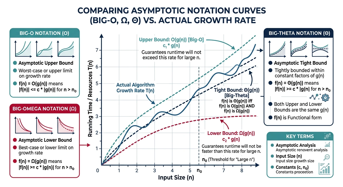
Graph comparing Big-O upper bound, Omega lower bound, and Theta tight bound notation curves against an algorithm's actual growth rate — Asymptotic Notations — Big-O provides the upper bound, Omega the lower bound, and Theta the tight bound of an algorithm's growth rate

Omega Notation (O) - Lower Bound

Describes the best-case scenario. "The algorithm takes at least this much time." Useful for proving minimum required work.

Theta Notation (T) - Tight Bound

When upper and lower bounds match. "The algorithm takes exactly this order of time." The most precise description.

# Understanding Asymptotic Notations through Search Algorithms
import time

def linear_search(arr, target):
    """
    Time Complexity Analysis:
    - Best Case O(1): target is at index 0
    - Worst Case O(n): target is last element or not present
    - Average Case T(n): target is somewhere in the middle
    """
    for i in range(len(arr)):
        if arr[i] == target:
            return i
    return -1

def binary_search(arr, target):
    """
    Time Complexity: T(log n) - tight bound
    Requires sorted array
    Halves search space each iteration
    """
    left, right = 0, len(arr) - 1
    while left <= right:
        mid = (left + right) // 2
        if arr[mid] == target:
            return mid
        elif arr[mid] < target:
            left = mid + 1
        else:
            right = mid - 1
    return -1

# Test and compare
arr = list(range(1, 1000001))  # 1 million elements

# Worst case for linear search
start = time.time()
linear_search(arr, 1000000)  # Search for last element
linear_time = time.time() - start

# Same search with binary search
start = time.time()
binary_search(arr, 1000000)
binary_time = time.time() - start

print(f"Linear Search (O(n)): {linear_time:.6f} seconds")
print(f"Binary Search (O(log n)): {binary_time:.6f} seconds")
print(f"Binary is ~{linear_time/binary_time:.0f}x faster!")

// Understanding Asymptotic Notations in C++
#include <iostream>
#include <vector>
#include <chrono>
using namespace std;

// Linear Search - O(n)
int linearSearch(const vector<int>& arr, int target) {
    for (int i = 0; i < arr.size(); i++) {
        if (arr[i] == target) return i;
    }
    return -1;
}

// Binary Search - O(log n)
int binarySearch(const vector<int>& arr, int target) {
    int left = 0, right = arr.size() - 1;
    while (left <= right) {
        int mid = left + (right - left) / 2;  // Avoid overflow
        if (arr[mid] == target) return mid;
        else if (arr[mid] < target) left = mid + 1;
        else right = mid - 1;
    }
    return -1;
}

int main() {
    // Create array of 1 million elements
    vector<int> arr(1000000);
    for (int i = 0; i < 1000000; i++) {
        arr[i] = i + 1;
    }
    
    // Benchmark linear search (worst case)
    auto start = chrono::high_resolution_clock::now();
    linearSearch(arr, 1000000);
    auto end = chrono::high_resolution_clock::now();
    auto linearTime = chrono::duration<double>(end - start).count();
    
    // Benchmark binary search
    start = chrono::high_resolution_clock::now();
    binarySearch(arr, 1000000);
    end = chrono::high_resolution_clock::now();
    auto binaryTime = chrono::duration<double>(end - start).count();
    
    cout << "Linear Search O(n): " << linearTime << " seconds" << endl;
    cout << "Binary Search O(log n): " << binaryTime << " seconds" << endl;
    cout << "Binary is ~" << (int)(linearTime/binaryTime) << "x faster!" << endl;
    
    return 0;
}

// Understanding Asymptotic Notations in Java
public class SearchComparison {
    
    // Linear Search - O(n)
    public static int linearSearch(int[] arr, int target) {
        for (int i = 0; i < arr.length; i++) {
            if (arr[i] == target) return i;
        }
        return -1;
    }
    
    // Binary Search - O(log n)
    public static int binarySearch(int[] arr, int target) {
        int left = 0, right = arr.length - 1;
        while (left <= right) {
            int mid = left + (right - left) / 2;  // Avoid overflow
            if (arr[mid] == target) return mid;
            else if (arr[mid] < target) left = mid + 1;
            else right = mid - 1;
        }
        return -1;
    }
    
    public static void main(String[] args) {
        // Create array of 1 million elements
        int[] arr = new int[1000000];
        for (int i = 0; i < 1000000; i++) {
            arr[i] = i + 1;
        }
        
        // Benchmark linear search (worst case)
        long start = System.nanoTime();
        linearSearch(arr, 1000000);
        long linearTime = System.nanoTime() - start;
        
        // Benchmark binary search
        start = System.nanoTime();
        binarySearch(arr, 1000000);
        long binaryTime = System.nanoTime() - start;
        
        System.out.printf("Linear Search O(n): %.6f seconds%n", linearTime / 1e9);
        System.out.printf("Binary Search O(log n): %.6f seconds%n", binaryTime / 1e9);
        System.out.printf("Binary is ~%dx faster!%n", linearTime / binaryTime);
    }
}

Time Complexity

Time complexity measures how the number of operations grows with input size.

Complexity	Name	n=10	n=100	n=1000	Example
\(O(1)\)	Constant	1	1	1	Array access
\(O(\log n)\)	Logarithmic	3	7	10	Binary search
\(O(n)\)	Linear	10	100	1000	Linear search
\(O(n \log n)\)	Linearithmic	33	664	9966	Merge sort
\(O(n^{2})\)	Quadratic	100	10,000	1,000,000	Bubble sort
O(2n)	Exponential	1024	10³°	8	Naive Fibonacci

Space Complexity

What is Space Complexity?

Space complexity measures how much extra memory an algorithm needs as input size grows. It includes:

Auxiliary Space: Extra space used by the algorithm (not including input)
Total Space: Input space + auxiliary space

# Space Complexity Examples in Python

# O(1) - Constant Space
def sum_array(arr):
    """Uses fixed amount of extra memory regardless of input size"""
    total = 0  # Only one variable, no matter how big arr is
    for num in arr:
        total += num
    return total

# O(n) - Linear Space
def duplicate_array(arr):
    """Creates new array proportional to input size"""
    result = []  # New list grows with input
    for num in arr:
        result.append(num)
    return result

# O(n) - Recursion Stack Space
def factorial(n):
    """Each recursive call adds to stack - O(n) space"""
    if n <= 1:
        return 1
    return n * factorial(n - 1)

# O(n²) - Quadratic Space
def create_adjacency_matrix(n):
    """Creates n×n matrix - n² space"""
    matrix = [[0] * n for _ in range(n)]
    return matrix

# Test
print(f"Sum (O(1) space): {sum_array([1,2,3,4,5])}")
print(f"Duplicate (O(n) space): {duplicate_array([1,2,3])}")
print(f"5x5 matrix (O(n²) space) created")

// Space Complexity Examples in C++
#include <iostream>
#include <vector>
using namespace std;

// O(1) - Constant Space
int sumArray(const vector<int>& arr) {
    int total = 0;  // Fixed space regardless of input
    for (int num : arr) {
        total += num;
    }
    return total;
}

// O(n) - Linear Space
vector<int> duplicateArray(const vector<int>& arr) {
    vector<int> result;  // Grows with input size
    for (int num : arr) {
        result.push_back(num);
    }
    return result;
}

// O(n) - Recursion Stack Space
int factorial(int n) {
    if (n <= 1) return 1;
    return n * factorial(n - 1);  // Each call uses stack space
}

// O(n²) - Quadratic Space
vector<vector<int>> createAdjacencyMatrix(int n) {
    vector<vector<int>> matrix(n, vector<int>(n, 0));
    return matrix;
}

int main() {
    vector<int> arr = {1, 2, 3, 4, 5};
    
    cout << "Sum (O(1) space): " << sumArray(arr) << endl;
    cout << "Duplicate (O(n) space): created " << duplicateArray(arr).size() << " elements" << endl;
    cout << "5x5 matrix (O(n²) space): created " << createAdjacencyMatrix(5).size() << "x5 matrix" << endl;
    
    return 0;
}

// Space Complexity Examples in Java
import java.util.*;

public class SpaceComplexity {
    
    // O(1) - Constant Space
    public static int sumArray(int[] arr) {
        int total = 0;  // Fixed space
        for (int num : arr) {
            total += num;
        }
        return total;
    }
    
    // O(n) - Linear Space
    public static int[] duplicateArray(int[] arr) {
        int[] result = new int[arr.length];  // New array same size as input
        for (int i = 0; i < arr.length; i++) {
            result[i] = arr[i];
        }
        return result;
    }
    
    // O(n) - Recursion Stack Space
    public static int factorial(int n) {
        if (n <= 1) return 1;
        return n * factorial(n - 1);  // Stack grows with n
    }
    
    // O(n²) - Quadratic Space
    public static int[][] createAdjacencyMatrix(int n) {
        int[][] matrix = new int[n][n];  // n×n = n² space
        return matrix;
    }
    
    public static void main(String[] args) {
        int[] arr = {1, 2, 3, 4, 5};
        
        System.out.println("Sum (O(1) space): " + sumArray(arr));
        System.out.println("Duplicate (O(n) space): created " + duplicateArray(arr).length + " elements");
        System.out.println("5x5 matrix (O(n²) space): created " + createAdjacencyMatrix(5).length + "x5 matrix");
    }
}

Analyzing Complexity from Code

Learn to look at code and determine its time/space complexity. These patterns appear constantly in interviews!

Visual guide mapping common code patterns like single loops, nested loops, and halving loops to their corresponding time complexities — Code Pattern to Complexity Mapping — recognizing loop structures to quickly determine \(O(n)\), \(O(n^{2})\), \(O(\log n)\), and \(O(n \log n)\) complexities

# Complexity Analysis Patterns

# Pattern 1: Single Loop ? O(n)
def single_loop(n):
    """One loop through n elements = O(n)"""
    count = 0
    for i in range(n):
        count += 1  # O(1) operation, done n times
    return count

# Pattern 2: Nested Loops ? O(n²)
def nested_loops(n):
    """Loop inside loop = O(n × n) = O(n²)"""
    count = 0
    for i in range(n):       # Outer: n times
        for j in range(n):   # Inner: n times each
            count += 1       # Total: n × n = n²
    return count

# Pattern 3: Loop with Halving ? O(log n)
def halving_loop(n):
    """Halve each iteration = O(log n)"""
    count = 0
    while n > 1:
        n = n // 2  # Halve the problem size
        count += 1
    return count

# Pattern 4: Nested Loop with Halving Inner ? O(n log n)
def n_log_n_pattern(n):
    """Linear outer × logarithmic inner = O(n log n)"""
    count = 0
    for i in range(n):        # n times
        j = n
        while j > 1:          # log n times
            j = j // 2
            count += 1
    return count

# Pattern 5: Two Different Inputs ? O(n × m)
def two_inputs(arr1, arr2):
    """Don't assume same size - use O(n × m)"""
    count = 0
    for a in arr1:      # n times
        for b in arr2:  # m times
            count += 1
    return count

print(f"Single loop (1000): {single_loop(1000)} iterations")
print(f"Nested loops (10): {nested_loops(10)} iterations")
print(f"Halving loop (1000): {halving_loop(1000)} iterations")
print(f"n log n (100): {n_log_n_pattern(100)} iterations")

// Complexity Analysis Patterns in C++
#include <iostream>
#include <cmath>
using namespace std;

// Pattern 1: Single Loop ? O(n)
int singleLoop(int n) {
    int count = 0;
    for (int i = 0; i < n; i++) {
        count++;  // n iterations
    }
    return count;
}

// Pattern 2: Nested Loops ? O(n²)
int nestedLoops(int n) {
    int count = 0;
    for (int i = 0; i < n; i++) {
        for (int j = 0; j < n; j++) {
            count++;  // n × n = n² iterations
        }
    }
    return count;
}

// Pattern 3: Loop with Halving ? O(log n)
int halvingLoop(int n) {
    int count = 0;
    while (n > 1) {
        n = n / 2;  // log2(n) iterations
        count++;
    }
    return count;
}

// Pattern 4: n log n Pattern
int nLogNPattern(int n) {
    int count = 0;
    for (int i = 0; i < n; i++) {     // n times
        for (int j = n; j > 1; j /= 2) {  // log n times
            count++;
        }
    }
    return count;
}

int main() {
    cout << "Single loop (1000): " << singleLoop(1000) << " iterations" << endl;
    cout << "Nested loops (10): " << nestedLoops(10) << " iterations" << endl;
    cout << "Halving loop (1000): " << halvingLoop(1000) << " iterations" << endl;
    cout << "n log n (100): " << nLogNPattern(100) << " iterations" << endl;
    
    return 0;
}

// Complexity Analysis Patterns in Java
public class ComplexityPatterns {
    
    // Pattern 1: Single Loop ? O(n)
    public static int singleLoop(int n) {
        int count = 0;
        for (int i = 0; i < n; i++) {
            count++;  // n iterations
        }
        return count;
    }
    
    // Pattern 2: Nested Loops ? O(n²)
    public static int nestedLoops(int n) {
        int count = 0;
        for (int i = 0; i < n; i++) {
            for (int j = 0; j < n; j++) {
                count++;  // n × n iterations
            }
        }
        return count;
    }
    
    // Pattern 3: Loop with Halving ? O(log n)
    public static int halvingLoop(int n) {
        int count = 0;
        while (n > 1) {
            n = n / 2;  // log2(n) iterations
            count++;
        }
        return count;
    }
    
    // Pattern 4: n log n Pattern
    public static int nLogNPattern(int n) {
        int count = 0;
        for (int i = 0; i < n; i++) {
            for (int j = n; j > 1; j /= 2) {
                count++;
            }
        }
        return count;
    }
    
    public static void main(String[] args) {
        System.out.println("Single loop (1000): " + singleLoop(1000) + " iterations");
        System.out.println("Nested loops (10): " + nestedLoops(10) + " iterations");
        System.out.println("Halving loop (1000): " + halvingLoop(1000) + " iterations");
        System.out.println("n log n (100): " + nLogNPattern(100) + " iterations");
    }
}

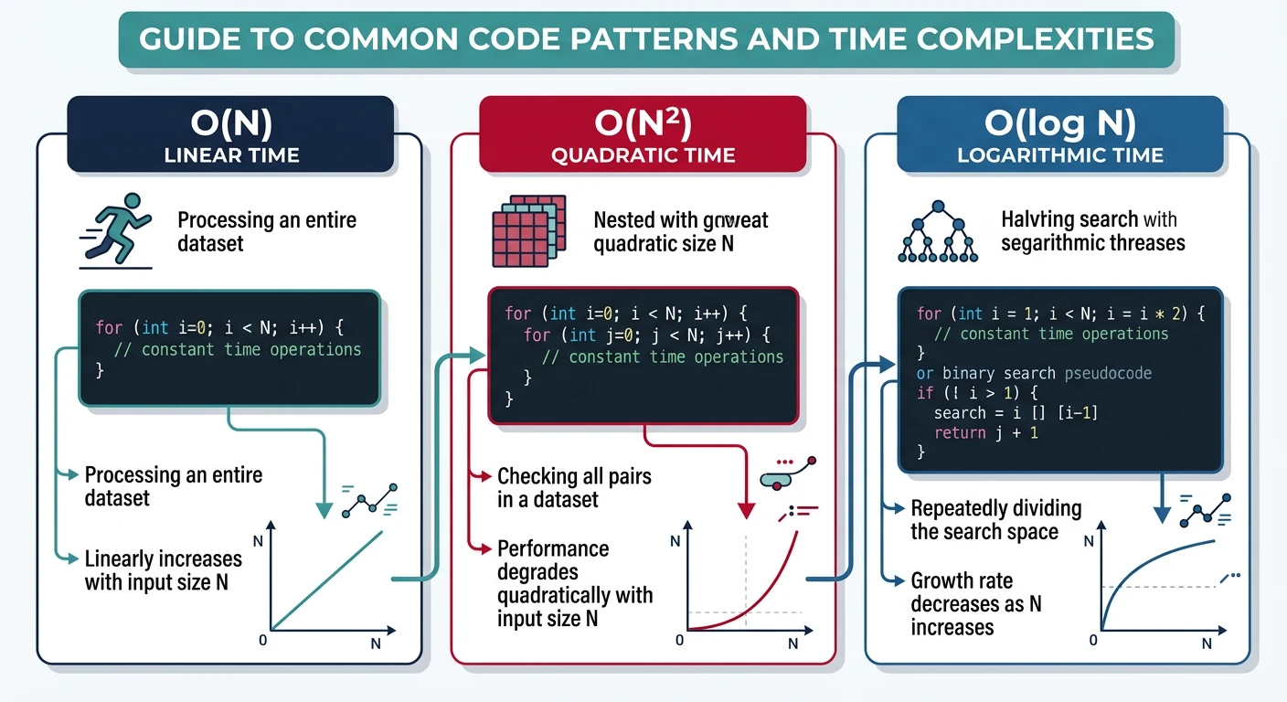
                            Complexity Rules Summary
                            Drop constants: O(2n) ? \(O(n)\), \(O(100n^{2})\) ? \(O(n^{2})\)
Drop lower-order terms: \(O(n^{2} + n)\) ? \(O(n^{2})\), O(n + log n) ? \(O(n)\)
Sequential operations: O(A) + O(B) = O(A + B) ? O(max(A, B))
Nested operations: O(A) × O(B) = O(A × B)
Different inputs, different variables: \(O(n \times m)\), not \(O(n^{2})\)

                        

LeetCode Practice Problems

Practice these foundational problems to solidify your understanding. Solutions provided in Python, C++, and Java!

Easy 1920. Build Array from Permutation

Given a zero-based permutation nums, build array ans where ans[i] = nums[nums[i]].

Analysis: Time \(O(n)\), Space \(O(n)\) - we create a new array of size n.

# LeetCode 1920 - Build Array from Permutation
# Time: O(n), Space: O(n)

def buildArray(nums):
    """Use list comprehension for clean Pythonic solution"""
    return [nums[nums[i]] for i in range(len(nums))]

# Test cases
print(buildArray([0,2,1,5,3,4]))  # Output: [0,1,2,4,5,3]
print(buildArray([5,0,1,2,3,4]))  # Output: [4,5,0,1,2,3]

// LeetCode 1920 - Build Array from Permutation
// Time: O(n), Space: O(n)
#include <vector>
#include <iostream>
using namespace std;

class Solution {
public:
    vector<int> buildArray(vector<int>& nums) {
        vector<int> ans(nums.size());
        for (int i = 0; i < nums.size(); i++) {
            ans[i] = nums[nums[i]];
        }
        return ans;
    }
};

int main() {
    Solution sol;
    vector<int> nums = {0, 2, 1, 5, 3, 4};
    vector<int> result = sol.buildArray(nums);
    
    for (int x : result) cout << x << " ";  // 0 1 2 4 5 3
    return 0;
}

// LeetCode 1920 - Build Array from Permutation
// Time: O(n), Space: O(n)
import java.util.Arrays;

class Solution {
    public int[] buildArray(int[] nums) {
        int[] ans = new int[nums.length];
        for (int i = 0; i < nums.length; i++) {
            ans[i] = nums[nums[i]];
        }
        return ans;
    }
    
    public static void main(String[] args) {
        Solution sol = new Solution();
        int[] nums = {0, 2, 1, 5, 3, 4};
        int[] result = sol.buildArray(nums);
        System.out.println(Arrays.toString(result));  // [0, 1, 2, 4, 5, 3]
    }
}

Easy 2011. Final Value After Operations

Given array of operations, perform ++X, X++, --X, X-- on initial X=0.

Analysis: Time \(O(n)\), Space \(O(1)\) - just iterate and check characters.

# LeetCode 2011 - Final Value After Operations
# Time: O(n), Space: O(1)

def finalValueAfterOperations(operations):
    """Check if '+' is in the operation string"""
    x = 0
    for op in operations:
        if '+' in op:
            x += 1
        else:
            x -= 1
    return x

# Test cases
print(finalValueAfterOperations(["--X","X++","X++"]))  # Output: 1
print(finalValueAfterOperations(["++X","++X","X++"]))  # Output: 3

// LeetCode 2011 - Final Value After Operations
// Time: O(n), Space: O(1)
#include <vector>
#include <string>
#include <iostream>
using namespace std;

class Solution {
public:
    int finalValueAfterOperations(vector<string>& operations) {
        int x = 0;
        for (const string& op : operations) {
            // Check if '+' exists in the operation string
            if (op.find('+') != string::npos) {
                x++;
            } else {
                x--;
            }
        }
        return x;
    }
};

int main() {
    Solution sol;
    vector<string> ops = {"--X", "X++", "X++"};
    cout << sol.finalValueAfterOperations(ops) << endl;  // Output: 1
    return 0;
}

// LeetCode 2011 - Final Value After Operations
// Time: O(n), Space: O(1)

class Solution {
    public int finalValueAfterOperations(String[] operations) {
        int x = 0;
        for (String op : operations) {
            if (op.contains("+")) {
                x++;
            } else {
                x--;
            }
        }
        return x;
    }
    
    public static void main(String[] args) {
        Solution sol = new Solution();
        String[] ops = {"--X", "X++", "X++"};
        System.out.println(sol.finalValueAfterOperations(ops));  // Output: 1
    }
}

Next in the Series

In Part 2: Recursion Complete Guide, we’ll master recursion patterns — the foundation for divide-and-conquer, tree traversals, and dynamic programming that powers the rest of this series.

Complete DSA Series Part 1: Foundations, Memory & Complexity

Table of Contents

FAANG Interview Prep

Foundations, Memory & Complexity

Recursion Complete Guide

Arrays & Array ADT

Strings

Matrices

Linked Lists

Stack

Queue

Trees

BST & Balanced Trees

Heaps, Sorting & Hashing

Graphs, DP, Greedy & Backtracking

Introduction: Why DSA Matters

Physical vs Logical Data Structures

Physical Data Structures

What are Data Structures?

Physical Data Structures

Logical Data Structures

Key Insight

Abstract Data Types (ADT)

What is an ADT?

List ADT Operations

Stack vs Heap Memory

Why Does Memory Matter?

Memory Management Comparison

Static vs Dynamic Memory Allocation

Static Allocation

Dynamic Allocation

Asymptotic Notations (O, O, T)

Why Asymptotic Notation?

The Three Notations

Big-O Notation (O) - Upper Bound

Omega Notation (O) - Lower Bound

Theta Notation (T) - Tight Bound

Time Complexity

Space Complexity

What is Space Complexity?

Analyzing Complexity from Code

Complexity Rules Summary

LeetCode Practice Problems

Easy 1920. Build Array from Permutation

Easy 2011. Final Value After Operations

Next in the Series

Continue the Series

Part 2: Recursion Complete Guide

Part 3: Arrays & Array ADT

Part 4: Strings