Arrays & Array ADT Operations: Complete DSA Guide with Python

FAANG Interview Prep

Your 12-step learning path • Currently on Step 3

Foundations, Memory & Complexity

Big-O notation, time/space analysis, memory layout

Recursion Complete Guide

Base cases, call stack, tail recursion, memoization

Arrays & Array ADT

Static/dynamic arrays, operations, amortized analysis

You Are Here

Introduction to Arrays

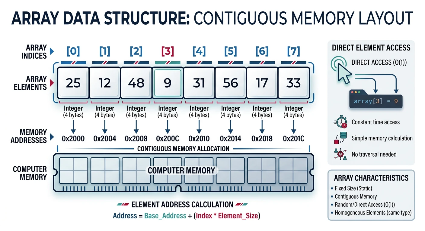
Arrays are the most fundamental data structure in computer science—a contiguous block of memory that stores elements of the same type. Understanding arrays deeply is essential because they form the foundation for implementing many other data structures.

Array data structure showing contiguous memory blocks with numbered indices and direct element access — Array Memory Layout — elements stored in contiguous memory blocks enabling \(O(1)\) random access by index

                            
                            Key Insight: Arrays provide \(O(1)\) random access by index, making them the fastest data structure for element retrieval. However, insertions and deletions require shifting elements, making these operations \(O(n)\).
                        

Static vs Dynamic Arrays

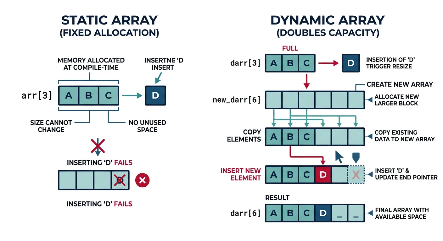
Arrays come in two flavors: static (fixed-size) and dynamic (resizable). Understanding both is crucial for interview success.

Comparison of static array with fixed allocation versus dynamic array that doubles capacity when full — Static vs Dynamic Arrays — static arrays have fixed size at creation while dynamic arrays automatically resize by doubling capacity

Aspect	Static Array	Dynamic Array
Size	Fixed at creation	Grows/shrinks automatically
Memory	Stack or heap	Always heap
Allocation	Compile-time or one-time	Runtime (may reallocate)
Append	N/A (fixed)	Amortized \(O(1)\)
Python	`array.array()`	`list`
C++	`int arr[n]` or `std::array`	`std::vector`
Java	`int[]`	`ArrayList`

# Static vs Dynamic Arrays in Python
import array
import sys

# STATIC: Fixed-size array using array module
# Type codes: 'i' = signed int, 'f' = float, 'd' = double
static_arr = array.array('i', [10, 20, 30, 40, 50])
print(f"Static array: {list(static_arr)}")
print(f"Type code: {static_arr.typecode}")
print(f"Item size: {static_arr.itemsize} bytes")

# Accessing elements: O(1)
print(f"Element at index 2: {static_arr[2]}")  # Output: 30

# DYNAMIC: Python list - automatically resizes
dynamic_arr = [10, 20, 30, 40, 50]

# Append operation: Amortized O(1)
dynamic_arr.append(60)
print(f"After append: {dynamic_arr}")  # [10, 20, 30, 40, 50, 60]

# Dynamic array capacity demonstration
sizes = []
prev_size = 0
arr = []
for i in range(100):
    arr.append(i)
    curr_size = sys.getsizeof(arr)
    if curr_size != prev_size:
        sizes.append((i, curr_size))
        prev_size = curr_size

print("\nDynamic array growth pattern:")
for count, size in sizes[:8]:
    print(f"  {count} elements: {size} bytes")

// Static vs Dynamic Arrays in C++
#include <iostream>
#include <array>
#include <vector>
using namespace std;

int main() {
    // STATIC ARRAY - Fixed size, stack allocated
    int staticArr[5] = {10, 20, 30, 40, 50};
    cout << "Static C-style array: ";
    for (int i = 0; i < 5; i++) {
        cout << staticArr[i] << " ";
    }
    cout << endl;
    
    // std::array - Modern C++ static array
    array<int, 5> stdArray = {10, 20, 30, 40, 50};
    cout << "std::array: ";
    for (int x : stdArray) {
        cout << x << " ";
    }
    cout << "\nstd::array size: " << stdArray.size() << endl;
    
    // DYNAMIC ARRAY - std::vector (resizable)
    vector<int> dynamicArr = {10, 20, 30, 40, 50};
    
    cout << "\nBefore append - Size: " << dynamicArr.size() 
         << ", Capacity: " << dynamicArr.capacity() << endl;
    
    // Append operation: Amortized O(1)
    dynamicArr.push_back(60);
    dynamicArr.push_back(70);
    
    cout << "After append - Size: " << dynamicArr.size() 
         << ", Capacity: " << dynamicArr.capacity() << endl;
    
    cout << "Vector contents: ";
    for (int x : dynamicArr) {
        cout << x << " ";
    }
    cout << endl;
    
    // Demonstrate capacity growth
    cout << "\nCapacity growth pattern:" << endl;
    vector<int> v;
    size_t prevCap = 0;
    for (int i = 0; i < 50; i++) {
        v.push_back(i);
        if (v.capacity() != prevCap) {
            cout << "  Size: " << v.size() 
                 << ", Capacity: " << v.capacity() << endl;
            prevCap = v.capacity();
        }
    }
    
    return 0;
}

// Static vs Dynamic Arrays in Java
import java.util.ArrayList;
import java.util.Arrays;

public class ArrayTypes {
    public static void main(String[] args) {
        // STATIC ARRAY - Fixed size
        int[] staticArr = {10, 20, 30, 40, 50};
        System.out.println("Static array: " + Arrays.toString(staticArr));
        System.out.println("Length: " + staticArr.length);
        System.out.println("Element at index 2: " + staticArr[2]);  // 30
        
        // Cannot resize static array - must create new one
        // staticArr.append() - NOT POSSIBLE
        
        // DYNAMIC ARRAY - ArrayList (resizable)
        ArrayList<Integer> dynamicArr = new ArrayList<>();
        dynamicArr.add(10);
        dynamicArr.add(20);
        dynamicArr.add(30);
        dynamicArr.add(40);
        dynamicArr.add(50);
        
        System.out.println("\nDynamic ArrayList: " + dynamicArr);
        System.out.println("Size: " + dynamicArr.size());
        
        // Append operation: Amortized O(1)
        dynamicArr.add(60);
        dynamicArr.add(70);
        System.out.println("After append: " + dynamicArr);
        
        // Access by index: O(1)
        System.out.println("Element at index 3: " + dynamicArr.get(3));
        
        // Insert at specific position: O(n)
        dynamicArr.add(2, 25);  // Insert 25 at index 2
        System.out.println("After insert at index 2: " + dynamicArr);
        
        // Remove by index: O(n)
        int removed = dynamicArr.remove(2);  // Remove element at index 2
        System.out.println("After remove at index 2: " + dynamicArr);
        System.out.println("Removed value: " + removed);
        
        // Convert between static and dynamic
        Integer[] backToStatic = dynamicArr.toArray(new Integer[0]);
        System.out.println("\nConverted back to array: " + Arrays.toString(backToStatic));
    }
}

Address Calculation

For a 1D array, the memory address of element at index i is calculated as:

Formula: Address(A[i]) = Base_Address + (i × Element_Size)

# Address Calculation Demonstration
import ctypes
import array

# Create an integer array
arr = array.array('i', [10, 20, 30, 40, 50])

# Get base address
base_address = arr.buffer_info()[0]
element_size = arr.itemsize  # 4 bytes for 'i' (integer)

print(f"Base address: {hex(base_address)}")
print(f"Element size: {element_size} bytes")

# Calculate addresses
for i in range(len(arr)):
    calculated_addr = base_address + (i * element_size)
    print(f"A[{i}] = {arr[i]:2d}, Address: {hex(calculated_addr)}")

# Python lists store references, not contiguous values
print("\nPython list (stores references):")
py_list = [10, 20, 30, 40, 50]
for i, val in enumerate(py_list):
    print(f"  Index {i}: value={val}, id={id(val)}")

// Address Calculation in C++
#include <iostream>
using namespace std;

int main() {
    int arr[] = {10, 20, 30, 40, 50};
    int n = sizeof(arr) / sizeof(arr[0]);
    
    // Get base address using pointer
    int* baseAddress = arr;  // or &arr[0]
    int elementSize = sizeof(int);  // 4 bytes on most systems
    
    cout << "Base address: " << baseAddress << endl;
    cout << "Element size: " << elementSize << " bytes" << endl;
    cout << endl;
    
    // Calculate and verify addresses
    for (int i = 0; i < n; i++) {
        // Calculated address using formula
        int* calculatedAddr = baseAddress + i;  // C++ handles multiplication
        
        cout << "A[" << i << "] = " << arr[i] 
             << ", Address: " << calculatedAddr << endl;
    }
    
    // Demonstrate pointer arithmetic
    cout << "\nPointer arithmetic demonstration:" << endl;
    cout << "&arr[0] = " << &arr[0] << endl;
    cout << "&arr[1] = " << &arr[1] << endl;
    cout << "Difference = " << (&arr[1] - &arr[0]) << " element(s)" << endl;
    cout << "Byte difference = " << ((char*)&arr[1] - (char*)&arr[0]) << " bytes" << endl;
    
    return 0;
}

// Address Calculation Concept in Java
// Note: Java abstracts memory addresses, but we can understand the concept

public class AddressCalculation {
    public static void main(String[] args) {
        int[] arr = {10, 20, 30, 40, 50};
        int elementSize = Integer.BYTES;  // 4 bytes
        
        System.out.println("Element size: " + elementSize + " bytes");
        System.out.println();
        
        // In Java, we can't get actual memory addresses
        // but the formula still applies internally:
        // Address(A[i]) = Base + (i × ElementSize)
        
        System.out.println("Conceptual address calculation:");
        int simulatedBase = 1000;  // Simulated base address
        
        for (int i = 0; i < arr.length; i++) {
            int simulatedAddr = simulatedBase + (i * elementSize);
            System.out.println("A[" + i + "] = " + arr[i] 
                             + ", Simulated Address: " + simulatedAddr);
        }
        
        // We can see hash codes (not actual addresses, but unique identifiers)
        System.out.println("\nArray reference hash: " + System.identityHashCode(arr));
        
        // For objects, each has its own identity
        Integer[] objArr = {10, 20, 30, 40, 50};
        System.out.println("\nObject array - each Integer has unique identity:");
        for (int i = 0; i < objArr.length; i++) {
            System.out.println("  objArr[" + i + "] = " + objArr[i] 
                             + ", hashCode: " + System.identityHashCode(objArr[i]));
        }
    }
}

Array ADT (Abstract Data Type)

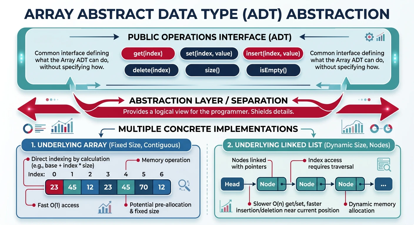
The Array ADT defines the operations we can perform on an array, independent of implementation. Let's build a complete Array ADT class in all three languages.

Diagram of Array ADT showing the abstraction layer between the operations interface and underlying array or linked list implementation — Array ADT Abstraction — the interface defines what operations are available while hiding how they are implemented internally

Array ADT Operations

display() - Show all elements
append(x) - Add element at end
insert(index, x) - Insert at position
delete(index) - Remove at position
search(x) - Find element (linear/binary)
get(index) - Get element at position
set(index, x) - Update element
max(), min(), sum(), avg() - Aggregate operations
reverse() - Reverse in place
is_sorted() - Check if sorted

# Complete Array ADT Implementation in Python
class ArrayADT:
    """Array Abstract Data Type with standard operations."""
    
    def __init__(self, capacity=10):
        self.capacity = capacity
        self.size = 0
        self.data = [None] * capacity
    
    def __len__(self):
        return self.size
    
    def __str__(self):
        return f"[{', '.join(str(self.data[i]) for i in range(self.size))}]"
    
    def display(self):
        """Print all elements. Time: O(n)"""
        for i in range(self.size):
            print(self.data[i], end=" ")
        print()
    
    def append(self, element):
        """Add element at end. Time: O(1) amortized"""
        if self.size >= self.capacity:
            self._resize(self.capacity * 2)
        self.data[self.size] = element
        self.size += 1
    
    def insert(self, index, element):
        """Insert at index. Time: O(n)"""
        if index < 0 or index > self.size:
            raise IndexError("Index out of bounds")
        if self.size >= self.capacity:
            self._resize(self.capacity * 2)
        for i in range(self.size, index, -1):
            self.data[i] = self.data[i - 1]
        self.data[index] = element
        self.size += 1
    
    def delete(self, index):
        """Delete at index. Time: O(n)"""
        if index < 0 or index >= self.size:
            raise IndexError("Index out of bounds")
        deleted = self.data[index]
        for i in range(index, self.size - 1):
            self.data[i] = self.data[i + 1]
        self.data[self.size - 1] = None
        self.size -= 1
        return deleted
    
    def get(self, index):
        """Get element. Time: O(1)"""
        if index < 0 or index >= self.size:
            raise IndexError("Index out of bounds")
        return self.data[index]
    
    def set(self, index, element):
        """Set element. Time: O(1)"""
        if index < 0 or index >= self.size:
            raise IndexError("Index out of bounds")
        self.data[index] = element
    
    def _resize(self, new_capacity):
        new_data = [None] * new_capacity
        for i in range(self.size):
            new_data[i] = self.data[i]
        self.data = new_data
        self.capacity = new_capacity
    
    def max(self):
        if self.size == 0: return None
        return max(self.data[i] for i in range(self.size))
    
    def min(self):
        if self.size == 0: return None
        return min(self.data[i] for i in range(self.size))
    
    def sum(self):
        return sum(self.data[i] for i in range(self.size))
    
    def avg(self):
        return self.sum() / self.size if self.size > 0 else 0

# Test
arr = ArrayADT(5)
for x in [10, 20, 30, 40, 50]:
    arr.append(x)
print(f"Array: {arr}")
print(f"Max: {arr.max()}, Min: {arr.min()}, Sum: {arr.sum()}")
arr.insert(2, 25)
print(f"After insert(2, 25): {arr}")

// Complete Array ADT Implementation in C++
#include <iostream>
#include <stdexcept>
using namespace std;

template <typename T>
class ArrayADT {
private:
    T* data;
    int capacity;
    int size;
    
    void resize(int newCapacity) {
        T* newData = new T[newCapacity];
        for (int i = 0; i < size; i++) {
            newData[i] = data[i];
        }
        delete[] data;
        data = newData;
        capacity = newCapacity;
    }

public:
    ArrayADT(int cap = 10) : capacity(cap), size(0) {
        data = new T[capacity];
    }
    
    ~ArrayADT() { delete[] data; }
    
    int length() const { return size; }
    
    void display() const {
        cout << "[";
        for (int i = 0; i < size; i++) {
            cout << data[i];
            if (i < size - 1) cout << ", ";
        }
        cout << "]" << endl;
    }
    
    void append(T element) {
        if (size >= capacity) resize(capacity * 2);
        data[size++] = element;
    }
    
    void insert(int index, T element) {
        if (index < 0 || index > size) 
            throw out_of_range("Index out of bounds");
        if (size >= capacity) resize(capacity * 2);
        for (int i = size; i > index; i--) {
            data[i] = data[i - 1];
        }
        data[index] = element;
        size++;
    }
    
    T remove(int index) {
        if (index < 0 || index >= size)
            throw out_of_range("Index out of bounds");
        T deleted = data[index];
        for (int i = index; i < size - 1; i++) {
            data[i] = data[i + 1];
        }
        size--;
        return deleted;
    }
    
    T get(int index) const {
        if (index < 0 || index >= size)
            throw out_of_range("Index out of bounds");
        return data[index];
    }
    
    void set(int index, T element) {
        if (index < 0 || index >= size)
            throw out_of_range("Index out of bounds");
        data[index] = element;
    }
    
    T max() const {
        if (size == 0) throw runtime_error("Empty array");
        T maxVal = data[0];
        for (int i = 1; i < size; i++) {
            if (data[i] > maxVal) maxVal = data[i];
        }
        return maxVal;
    }
    
    T min() const {
        if (size == 0) throw runtime_error("Empty array");
        T minVal = data[0];
        for (int i = 1; i < size; i++) {
            if (data[i] < minVal) minVal = data[i];
        }
        return minVal;
    }
    
    T sum() const {
        T total = 0;
        for (int i = 0; i < size; i++) total += data[i];
        return total;
    }
};

int main() {
    ArrayADT<int> arr(5);
    arr.append(10); arr.append(20); arr.append(30);
    arr.append(40); arr.append(50);
    
    cout << "Array: "; arr.display();
    cout << "Max: " << arr.max() << ", Min: " << arr.min() 
         << ", Sum: " << arr.sum() << endl;
    
    arr.insert(2, 25);
    cout << "After insert(2, 25): "; arr.display();
    
    return 0;
}

// Complete Array ADT Implementation in Java
public class ArrayADT<T extends Comparable<T>> {
    private Object[] data;
    private int capacity;
    private int size;
    
    public ArrayADT(int capacity) {
        this.capacity = capacity;
        this.size = 0;
        this.data = new Object[capacity];
    }
    
    public int length() { return size; }
    
    public void display() {
        System.out.print("[");
        for (int i = 0; i < size; i++) {
            System.out.print(data[i]);
            if (i < size - 1) System.out.print(", ");
        }
        System.out.println("]");
    }
    
    public void append(T element) {
        if (size >= capacity) resize(capacity * 2);
        data[size++] = element;
    }
    
    public void insert(int index, T element) {
        if (index < 0 || index > size)
            throw new IndexOutOfBoundsException("Index out of bounds");
        if (size >= capacity) resize(capacity * 2);
        for (int i = size; i > index; i--) {
            data[i] = data[i - 1];
        }
        data[index] = element;
        size++;
    }
    
    @SuppressWarnings("unchecked")
    public T remove(int index) {
        if (index < 0 || index >= size)
            throw new IndexOutOfBoundsException("Index out of bounds");
        T deleted = (T) data[index];
        for (int i = index; i < size - 1; i++) {
            data[i] = data[i + 1];
        }
        size--;
        return deleted;
    }
    
    @SuppressWarnings("unchecked")
    public T get(int index) {
        if (index < 0 || index >= size)
            throw new IndexOutOfBoundsException("Index out of bounds");
        return (T) data[index];
    }
    
    public void set(int index, T element) {
        if (index < 0 || index >= size)
            throw new IndexOutOfBoundsException("Index out of bounds");
        data[index] = element;
    }
    
    private void resize(int newCapacity) {
        Object[] newData = new Object[newCapacity];
        for (int i = 0; i < size; i++) newData[i] = data[i];
        data = newData;
        capacity = newCapacity;
    }
    
    @SuppressWarnings("unchecked")
    public T max() {
        if (size == 0) return null;
        T maxVal = (T) data[0];
        for (int i = 1; i < size; i++) {
            if (((T) data[i]).compareTo(maxVal) > 0) maxVal = (T) data[i];
        }
        return maxVal;
    }
    
    @SuppressWarnings("unchecked")
    public T min() {
        if (size == 0) return null;
        T minVal = (T) data[0];
        for (int i = 1; i < size; i++) {
            if (((T) data[i]).compareTo(minVal) < 0) minVal = (T) data[i];
        }
        return minVal;
    }
    
    public static void main(String[] args) {
        ArrayADT<Integer> arr = new ArrayADT<>(5);
        arr.append(10); arr.append(20); arr.append(30);
        arr.append(40); arr.append(50);
        
        System.out.print("Array: "); arr.display();
        System.out.println("Max: " + arr.max() + ", Min: " + arr.min());
        
        arr.insert(2, 25);
        System.out.print("After insert(2, 25): "); arr.display();
    }
}

Insert & Delete Operations

Understanding insertion and deletion is crucial—these operations form the basis for many interview questions.

Step-by-step visualization of element shifting during array insertion at index and deletion from index — Array Insert & Delete Operations — inserting requires shifting elements right, deleting requires shifting elements left

Insertion at Different Positions

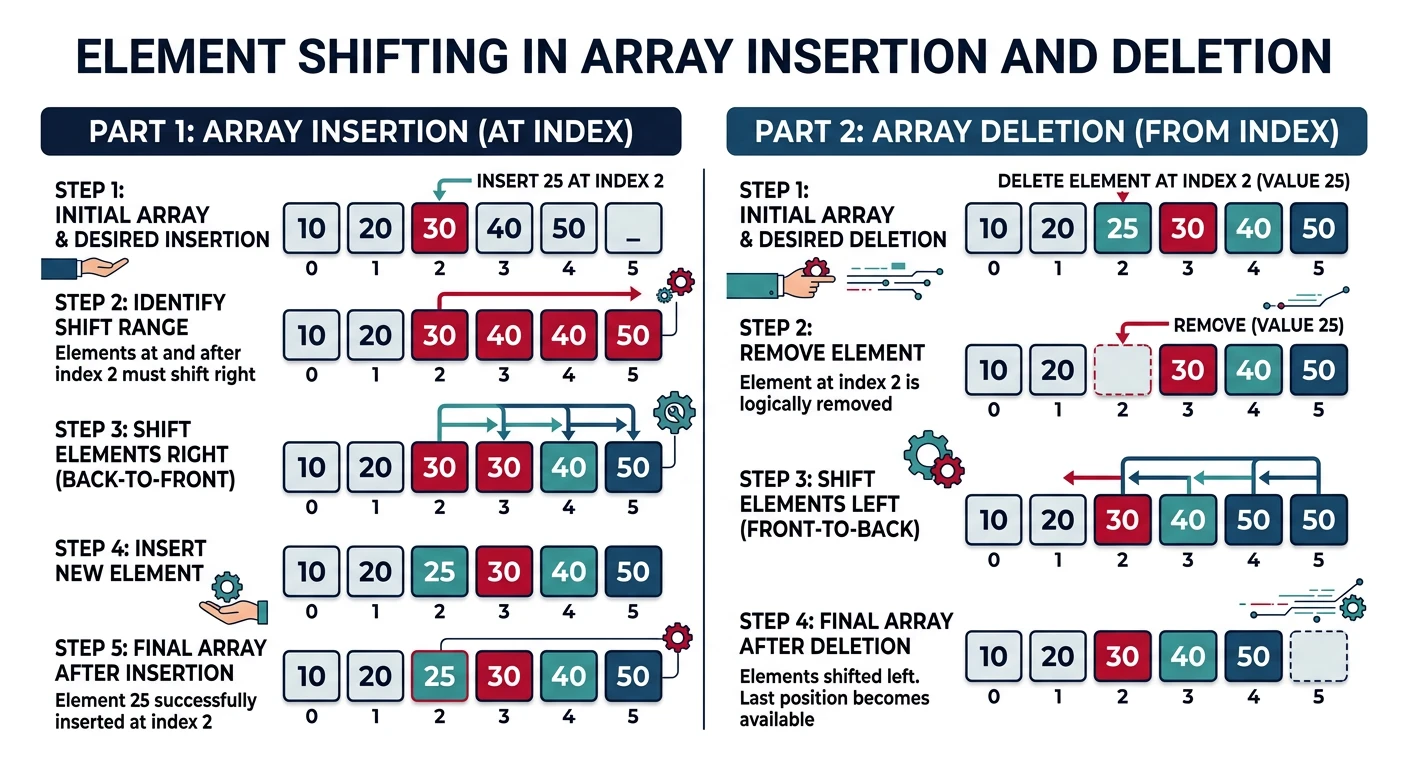
Inserting into an array requires shifting elements to make room. Inserting at the end (append) is \(O(1)\) amortized — no shifting needed, just place at the next available index. Inserting at the beginning is \(O(n)\) — every existing element must shift right by one position. Inserting at index \(k\) is \(O(n-k)\). This shifting cost is the fundamental tradeoff of arrays vs linked lists: arrays give \(O(1)\) random access but \(O(n)\) insertion/deletion in the middle.

# Insert Operations Visualization
class ArrayInsert:
    """Demonstrates different insertion scenarios"""
    
    def __init__(self, elements):
        self.arr = list(elements)
    
    def insert_at_beginning(self, element):
        """Insert at index 0. Time: O(n) - shift all elements"""
        # Shift all elements right by 1
        self.arr = [element] + self.arr
        return self.arr
    
    def insert_at_end(self, element):
        """Insert at last index. Time: O(1) amortized"""
        self.arr.append(element)
        return self.arr
    
    def insert_at_index(self, index, element):
        """Insert at specific index. Time: O(n-index)"""
        # Manual implementation showing the shift
        new_arr = []
        for i in range(len(self.arr) + 1):
            if i < index:
                new_arr.append(self.arr[i])
            elif i == index:
                new_arr.append(element)
            else:
                new_arr.append(self.arr[i-1])
        self.arr = new_arr
        return self.arr
    
    def insert_in_sorted(self, element):
        """Insert maintaining sorted order. Time: O(n)"""
        # Find correct position
        pos = 0
        for i in range(len(self.arr)):
            if self.arr[i] < element:
                pos = i + 1
            else:
                break
        
        # Insert at position
        self.arr.insert(pos, element)
        return self.arr

# Test insertions
arr = ArrayInsert([10, 20, 30, 40, 50])
print(f"Original: {arr.arr}")

# Insert at beginning - O(n)
arr = ArrayInsert([10, 20, 30, 40, 50])
print(f"Insert 5 at beginning: {arr.insert_at_beginning(5)}")

# Insert at end - O(1)
arr = ArrayInsert([10, 20, 30, 40, 50])
print(f"Insert 60 at end: {arr.insert_at_end(60)}")

# Insert at index 2 - O(n-2)
arr = ArrayInsert([10, 20, 30, 40, 50])
print(f"Insert 25 at index 2: {arr.insert_at_index(2, 25)}")

# Insert in sorted array - O(n)
arr = ArrayInsert([10, 20, 30, 40, 50])
print(f"Insert 35 in sorted: {arr.insert_in_sorted(35)}")

Deletion at Different Positions

Deletion is the mirror of insertion: removing from the end is \(O(1)\) (just decrement size), but removing from the beginning or middle requires shifting all subsequent elements left to fill the gap — \(O(n)\) worst case. An important optimization: if order doesn't matter, swap the target element with the last element and delete from the end — achieving \(O(1)\) deletion at any position.

# Delete Operations Visualization  
class ArrayDelete:
    """Demonstrates different deletion scenarios"""
    
    def __init__(self, elements):
        self.arr = list(elements)
    
    def delete_at_beginning(self):
        """Delete at index 0. Time: O(n) - shift all elements"""
        if not self.arr:
            return None
        deleted = self.arr[0]
        self.arr = self.arr[1:]
        return deleted, self.arr
    
    def delete_at_end(self):
        """Delete at last index. Time: O(1)"""
        if not self.arr:
            return None
        deleted = self.arr.pop()
        return deleted, self.arr
    
    def delete_at_index(self, index):
        """Delete at specific index. Time: O(n-index)"""
        if index < 0 or index >= len(self.arr):
            return None, self.arr
        
        deleted = self.arr[index]
        # Manual shift to show operation
        new_arr = []
        for i in range(len(self.arr)):
            if i != index:
                new_arr.append(self.arr[i])
        self.arr = new_arr
        return deleted, self.arr
    
    def delete_by_value(self, value):
        """Delete first occurrence of value. Time: O(n)"""
        for i in range(len(self.arr)):
            if self.arr[i] == value:
                deleted = self.arr[i]
                self.arr = self.arr[:i] + self.arr[i+1:]
                return deleted, self.arr
        return None, self.arr

# Test deletions
arr = ArrayDelete([10, 20, 30, 40, 50])
print(f"Original: {arr.arr}")

# Delete at beginning - O(n)
arr = ArrayDelete([10, 20, 30, 40, 50])
deleted, result = arr.delete_at_beginning()
print(f"Delete at beginning: {result}, Deleted: {deleted}")

# Delete at end - O(1)
arr = ArrayDelete([10, 20, 30, 40, 50])
deleted, result = arr.delete_at_end()
print(f"Delete at end: {result}, Deleted: {deleted}")

# Delete at index 2 - O(n-2)
arr = ArrayDelete([10, 20, 30, 40, 50])
deleted, result = arr.delete_at_index(2)
print(f"Delete at index 2: {result}, Deleted: {deleted}")

# Delete by value - O(n)
arr = ArrayDelete([10, 20, 30, 40, 50])
deleted, result = arr.delete_by_value(30)
print(f"Delete value 30: {result}, Deleted: {deleted}")

Searching Algorithms

Linear Search

Linear search examines each element sequentially until the target is found or the array ends. Works on any array (sorted or unsorted).

Case	Time Complexity	When
Best	\(O(1)\)	Element at first position
Average	O(n/2) = \(O(n)\)	Element in middle
Worst	\(O(n)\)	Element at last or not found

# Linear Search Variations in Python
def linear_search_basic(arr, target):
    """Basic linear search. Time: O(n), Space: O(1)"""
    for i in range(len(arr)):
        if arr[i] == target:
            return i
    return -1

def linear_search_transposition(arr, target):
    """Move found element one position towards front."""
    for i in range(len(arr)):
        if arr[i] == target:
            if i > 0:
                arr[i], arr[i-1] = arr[i-1], arr[i]
                return i - 1
            return i
    return -1

# Test
arr = [10, 20, 30, 40, 50, 60, 70]
print(f"Array: {arr}")
print(f"Search 40: index {linear_search_basic(arr, 40)}")
print(f"Search 100: index {linear_search_basic(arr, 100)}")

// Linear Search in C++
#include <iostream>
#include <vector>
using namespace std;

// Basic linear search - O(n) time, O(1) space
int linearSearch(const vector<int>& arr, int target) {
    for (int i = 0; i < arr.size(); i++) {
        if (arr[i] == target) {
            return i;
        }
    }
    return -1;
}

// Linear search with transposition optimization
int linearSearchTransposition(vector<int>& arr, int target) {
    for (int i = 0; i < arr.size(); i++) {
        if (arr[i] == target) {
            if (i > 0) {
                swap(arr[i], arr[i-1]);
                return i - 1;
            }
            return i;
        }
    }
    return -1;
}

int main() {
    vector<int> arr = {10, 20, 30, 40, 50, 60, 70};
    
    cout << "Array: ";
    for (int x : arr) cout << x << " ";
    cout << endl;
    
    cout << "Search 40: index " << linearSearch(arr, 40) << endl;
    cout << "Search 100: index " << linearSearch(arr, 100) << endl;
    
    return 0;
}

// Linear Search in Java
import java.util.Arrays;

public class LinearSearch {
    // Basic linear search - O(n) time, O(1) space
    public static int linearSearch(int[] arr, int target) {
        for (int i = 0; i < arr.length; i++) {
            if (arr[i] == target) {
                return i;
            }
        }
        return -1;
    }
    
    // Linear search with transposition optimization
    public static int linearSearchTransposition(int[] arr, int target) {
        for (int i = 0; i < arr.length; i++) {
            if (arr[i] == target) {
                if (i > 0) {
                    // Swap with previous element
                    int temp = arr[i];
                    arr[i] = arr[i - 1];
                    arr[i - 1] = temp;
                    return i - 1;
                }
                return i;
            }
        }
        return -1;
    }
    
    public static void main(String[] args) {
        int[] arr = {10, 20, 30, 40, 50, 60, 70};
        
        System.out.println("Array: " + Arrays.toString(arr));
        System.out.println("Search 40: index " + linearSearch(arr, 40));
        System.out.println("Search 100: index " + linearSearch(arr, 100));
    }
}

Binary Search

Binary search requires a sorted array and works by repeatedly dividing the search space in half. This is a fundamental algorithm you must master for FAANG interviews.

                            
                            Critical: Binary search only works on sorted arrays. Always verify the array is sorted or sort it first (adding \(O(n \log n)\) cost).
                        

# Binary Search in Python - Iterative & Recursive
def binary_search_iterative(arr, target):
    """Iterative binary search. Time: O(log n), Space: O(1)"""
    left, right = 0, len(arr) - 1
    
    while left <= right:
        mid = left + (right - left) // 2  # Avoid overflow
        
        if arr[mid] == target:
            return mid
        elif arr[mid] < target:
            left = mid + 1
        else:
            right = mid - 1
    return -1

def binary_search_recursive(arr, target, left, right):
    """Recursive binary search. Time: O(log n), Space: O(log n)"""
    if left > right:
        return -1
    
    mid = left + (right - left) // 2
    
    if arr[mid] == target:
        return mid
    elif arr[mid] < target:
        return binary_search_recursive(arr, target, mid + 1, right)
    else:
        return binary_search_recursive(arr, target, left, mid - 1)

# Test
arr = [10, 20, 30, 40, 50, 60, 70]
print(f"Array: {arr}")
print(f"Iterative search for 40: index {binary_search_iterative(arr, 40)}")
print(f"Recursive search for 40: index {binary_search_recursive(arr, 40, 0, len(arr)-1)}")
print(f"Search for 35 (not found): index {binary_search_iterative(arr, 35)}")

// Binary Search in C++ - Iterative & Recursive
#include <iostream>
#include <vector>
using namespace std;

// Iterative binary search - O(log n) time, O(1) space
int binarySearchIterative(const vector<int>& arr, int target) {
    int left = 0, right = arr.size() - 1;
    
    while (left <= right) {
        int mid = left + (right - left) / 2;  // Avoid overflow
        
        if (arr[mid] == target) {
            return mid;
        } else if (arr[mid] < target) {
            left = mid + 1;
        } else {
            right = mid - 1;
        }
    }
    return -1;
}

// Recursive binary search - O(log n) time, O(log n) space
int binarySearchRecursive(const vector<int>& arr, int target, int left, int right) {
    if (left > right) {
        return -1;
    }
    
    int mid = left + (right - left) / 2;
    
    if (arr[mid] == target) {
        return mid;
    } else if (arr[mid] < target) {
        return binarySearchRecursive(arr, target, mid + 1, right);
    } else {
        return binarySearchRecursive(arr, target, left, mid - 1);
    }
}

int main() {
    vector<int> arr = {10, 20, 30, 40, 50, 60, 70};
    
    cout << "Array: ";
    for (int x : arr) cout << x << " ";
    cout << endl;
    
    cout << "Iterative search for 40: index " 
         << binarySearchIterative(arr, 40) << endl;
    cout << "Recursive search for 40: index " 
         << binarySearchRecursive(arr, 40, 0, arr.size() - 1) << endl;
    cout << "Search for 35 (not found): index " 
         << binarySearchIterative(arr, 35) << endl;
    
    return 0;
}

// Binary Search in Java - Iterative & Recursive
import java.util.Arrays;

public class BinarySearch {
    // Iterative binary search - O(log n) time, O(1) space
    public static int binarySearchIterative(int[] arr, int target) {
        int left = 0, right = arr.length - 1;
        
        while (left <= right) {
            int mid = left + (right - left) / 2;  // Avoid overflow
            
            if (arr[mid] == target) {
                return mid;
            } else if (arr[mid] < target) {
                left = mid + 1;
            } else {
                right = mid - 1;
            }
        }
        return -1;
    }
    
    // Recursive binary search - O(log n) time, O(log n) space
    public static int binarySearchRecursive(int[] arr, int target, int left, int right) {
        if (left > right) {
            return -1;
        }
        
        int mid = left + (right - left) / 2;
        
        if (arr[mid] == target) {
            return mid;
        } else if (arr[mid] < target) {
            return binarySearchRecursive(arr, target, mid + 1, right);
        } else {
            return binarySearchRecursive(arr, target, left, mid - 1);
        }
    }
    
    public static void main(String[] args) {
        int[] arr = {10, 20, 30, 40, 50, 60, 70};
        
        System.out.println("Array: " + Arrays.toString(arr));
        System.out.println("Iterative search for 40: index " 
                         + binarySearchIterative(arr, 40));
        System.out.println("Recursive search for 40: index " 
                         + binarySearchRecursive(arr, 40, 0, arr.length - 1));
        System.out.println("Search for 35 (not found): index " 
                         + binarySearchIterative(arr, 35));
    }
}

Binary Search Interview Patterns

These advanced patterns appear frequently in FAANG interviews.

Python - First/Last Occurrence & Rotated Array

# Advanced Binary Search Patterns
def find_first_occurrence(arr, target):
    """Find first occurrence in sorted array with duplicates."""
    left, right = 0, len(arr) - 1
    result = -1
    
    while left <= right:
        mid = left + (right - left) // 2
        if arr[mid] == target:
            result = mid
            right = mid - 1  # Keep searching left
        elif arr[mid] < target:
            left = mid + 1
        else:
            right = mid - 1
    return result

def search_rotated_array(arr, target):
    """Search in rotated sorted array - Classic FAANG question!"""
    left, right = 0, len(arr) - 1
    
    while left <= right:
        mid = left + (right - left) // 2
        
        if arr[mid] == target:
            return mid
        
        # Left half is sorted
        if arr[left] <= arr[mid]:
            if arr[left] <= target < arr[mid]:
                right = mid - 1
            else:
                left = mid + 1
        # Right half is sorted
        else:
            if arr[mid] < target <= arr[right]:
                left = mid + 1
            else:
                right = mid - 1
    return -1

# Test
arr = [10, 20, 30, 30, 30, 40, 50]
print(f"First occurrence of 30: index {find_first_occurrence(arr, 30)}")

rotated = [40, 50, 60, 10, 20, 30]
print(f"Rotated array: {rotated}")
print(f"Search 10: index {search_rotated_array(rotated, 10)}")

2D Arrays & Matrices

2D arrays (matrices) are essential for many problems: grid traversals, dynamic programming, image processing, and graph adjacency matrices.

2D array memory layout showing row-major versus column-major ordering with address calculation formulas — 2D Array Memory Layout — row-major order stores rows contiguously (C, Python, Java) while column-major stores columns contiguously (Fortran, MATLAB)

# 2D Array Fundamentals
# Creating 2D arrays in Python

# Method 1: List comprehension (CORRECT)
rows, cols = 3, 4
matrix = [[0 for _ in range(cols)] for _ in range(rows)]
print("Empty 3x4 matrix:")
for row in matrix:
    print(row)

# Method 2: Direct initialization
matrix = [
    [1, 2, 3, 4],
    [5, 6, 7, 8],
    [9, 10, 11, 12]
]
print("\nInitialized matrix:")
for row in matrix:
    print(row)

# WRONG WAY (creates references, not copies!)
wrong_matrix = [[0] * cols] * rows
wrong_matrix[0][0] = 1  # This changes ALL rows!
print("\nWrong initialization (all rows share reference):")
for row in wrong_matrix:
    print(row)

# Accessing elements
print(f"\nElement at [1][2]: {matrix[1][2]}")  # Output: 7

# Iterating 2D arrays
print("\nRow-wise iteration:")
for i in range(len(matrix)):
    for j in range(len(matrix[0])):
        print(f"matrix[{i}][{j}] = {matrix[i][j]}")

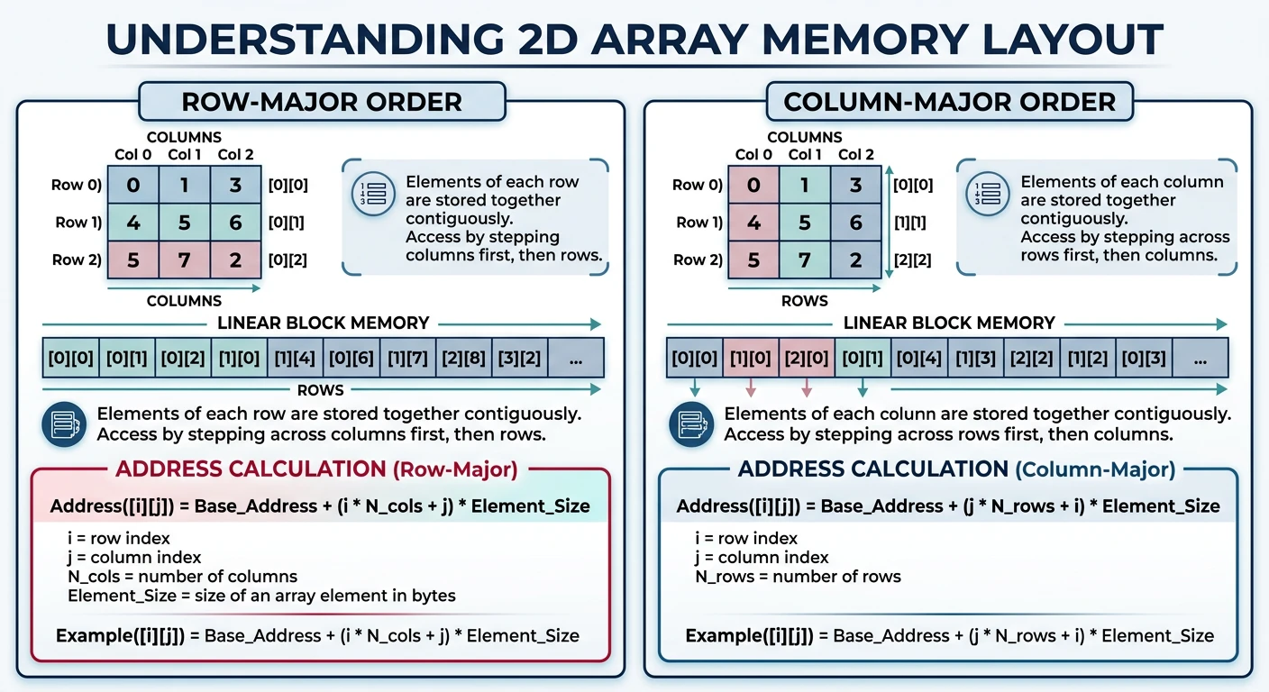
Row-Major vs Column-Major Ordering

Since memory is fundamentally 1-dimensional, 2D arrays must be linearized. Two conventions exist: Row-major (C, Java, Python) stores rows contiguously — elements in the same row are adjacent in memory. Column-major (Fortran, MATLAB, R) stores columns contiguously. This matters enormously for performance: traversing in the "natural" order of your language gives cache hits; traversing perpendicular to it causes cache misses. In C/Java, iterate rows in the outer loop; in Fortran/MATLAB, iterate columns first.

Address formula (row-major): For an \(m \times n\) matrix stored at base address \(B\), element \([i][j]\) is at \(B + (i \times n + j) \times \text{element\_size}\). Column-major swaps the roles: \(B + (j \times m + i) \times \text{element\_size}\).

Understanding memory layout is crucial for performance optimization and interview questions about index calculation.

Memory Layout

Row-Major (C, Python, Java): Elements of each row stored contiguously
Column-Major (Fortran, MATLAB): Elements of each column stored contiguously

# Row-Major vs Column-Major Address Calculation
def row_major_address(base, i, j, num_cols, element_size):
    """
    Calculate address in row-major order.
    Formula: Base + (i * num_cols + j) * element_size
    """
    return base + (i * num_cols + j) * element_size

def column_major_address(base, i, j, num_rows, element_size):
    """
    Calculate address in column-major order.
    Formula: Base + (j * num_rows + i) * element_size
    """
    return base + (j * num_rows + i) * element_size

# Example: 3x4 matrix
num_rows, num_cols = 3, 4
base_address = 1000
element_size = 4  # 4 bytes for integer

print("3x4 Matrix Address Calculation")
print("=" * 50)

# Create visual matrix
matrix = [[i * num_cols + j for j in range(num_cols)] for i in range(num_rows)]
print("\nLogical matrix indices:")
for row in matrix:
    print(row)

# Row-major layout
print("\nRow-Major Order (C, Python, Java):")
print("Memory: ", end="")
for i in range(num_rows):
    for j in range(num_cols):
        addr = row_major_address(base_address, i, j, num_cols, element_size)
        print(f"[{i},{j}]:{addr}", end=" ")
print()

# Column-major layout  
print("\nColumn-Major Order (Fortran, MATLAB):")
print("Memory: ", end="")
for j in range(num_cols):
    for i in range(num_rows):
        addr = column_major_address(base_address, i, j, num_rows, element_size)
        print(f"[{i},{j}]:{addr}", end=" ")
print()

# Performance implication
print("\n" + "=" * 50)
print("Performance Implication:")
print("Row-major: Access row-by-row for cache efficiency")
print("Column-major: Access column-by-column for cache efficiency")

2D Array Operations

# Common 2D Array Operations
import copy

class Matrix:
    """Matrix class with common operations"""
    
    def __init__(self, data):
        self.data = [row[:] for row in data]  # Deep copy
        self.rows = len(data)
        self.cols = len(data[0]) if data else 0
    
    def display(self):
        """Display matrix"""
        for row in self.data:
            print([f"{x:3}" for x in row])
        print()
    
    def transpose(self):
        """
        Transpose matrix (swap rows and columns).
        Time: O(rows × cols)
        """
        result = [[self.data[j][i] for j in range(self.rows)] 
                  for i in range(self.cols)]
        return Matrix(result)
    
    def rotate_90_clockwise(self):
        """
        Rotate 90° clockwise.
        Pattern: Transpose + Reverse each row
        Time: O(n²) for n×n matrix
        """
        # Transpose
        transposed = [[self.data[j][i] for j in range(self.rows)] 
                      for i in range(self.cols)]
        # Reverse each row
        for row in transposed:
            row.reverse()
        return Matrix(transposed)
    
    def rotate_90_counter_clockwise(self):
        """
        Rotate 90° counter-clockwise.
        Pattern: Transpose + Reverse each column
        Time: O(n²) for n×n matrix
        """
        # Transpose
        transposed = [[self.data[j][i] for j in range(self.rows)] 
                      for i in range(self.cols)]
        # Reverse the list of rows
        transposed.reverse()
        return Matrix(transposed)
    
    def spiral_order(self):
        """
        Return elements in spiral order.
        Classic interview question!
        Time: O(rows × cols)
        """
        if not self.data:
            return []
        
        result = []
        top, bottom = 0, self.rows - 1
        left, right = 0, self.cols - 1
        
        while top <= bottom and left <= right:
            # Right
            for j in range(left, right + 1):
                result.append(self.data[top][j])
            top += 1
            
            # Down
            for i in range(top, bottom + 1):
                result.append(self.data[i][right])
            right -= 1
            
            # Left
            if top <= bottom:
                for j in range(right, left - 1, -1):
                    result.append(self.data[bottom][j])
                bottom -= 1
            
            # Up
            if left <= right:
                for i in range(bottom, top - 1, -1):
                    result.append(self.data[i][left])
                left += 1
        
        return result

# Test matrix operations
matrix = Matrix([
    [1, 2, 3],
    [4, 5, 6],
    [7, 8, 9]
])

print("Original Matrix:")
matrix.display()

print("Transpose:")
matrix.transpose().display()

print("Rotate 90° Clockwise:")
matrix.rotate_90_clockwise().display()

print("Rotate 90° Counter-Clockwise:")
matrix.rotate_90_counter_clockwise().display()

print(f"Spiral Order: {matrix.spiral_order()}")

# 4x4 spiral example
matrix4 = Matrix([
    [1, 2, 3, 4],
    [5, 6, 7, 8],
    [9, 10, 11, 12],
    [13, 14, 15, 16]
])
print("\n4x4 Matrix Spiral Order:")
matrix4.display()
print(f"Spiral: {matrix4.spiral_order()}")

LeetCode Practice Problems

Practice these array problems to build strong foundations. Solutions provided in Python, C++, and Java!

Easy 704. Binary Search

Given sorted array, return index of target or -1.

# LeetCode 704 - Binary Search
# Time: O(log n), Space: O(1)

def search(nums, target):
    left, right = 0, len(nums) - 1
    while left <= right:
        mid = left + (right - left) // 2
        if nums[mid] == target:
            return mid
        elif nums[mid] < target:
            left = mid + 1
        else:
            right = mid - 1
    return -1

print(search([-1,0,3,5,9,12], 9))   # Output: 4

// LeetCode 704 - Binary Search
class Solution {
public:
    int search(vector<int>& nums, int target) {
        int left = 0, right = nums.size() - 1;
        while (left <= right) {
            int mid = left + (right - left) / 2;
            if (nums[mid] == target) return mid;
            else if (nums[mid] < target) left = mid + 1;
            else right = mid - 1;
        }
        return -1;
    }
};

// LeetCode 704 - Binary Search
class Solution {
    public int search(int[] nums, int target) {
        int left = 0, right = nums.length - 1;
        while (left <= right) {
            int mid = left + (right - left) / 2;
            if (nums[mid] == target) return mid;
            else if (nums[mid] < target) left = mid + 1;
            else right = mid - 1;
        }
        return -1;
    }
}

Easy 35. Search Insert Position

Find index to insert target in sorted array.

# LeetCode 35 - Search Insert Position
# Time: O(log n), Space: O(1)

def searchInsert(nums, target):
    left, right = 0, len(nums)
    while left < right:
        mid = left + (right - left) // 2
        if nums[mid] < target:
            left = mid + 1
        else:
            right = mid
    return left

print(searchInsert([1,3,5,6], 5))  # Output: 2
print(searchInsert([1,3,5,6], 2))  # Output: 1

// LeetCode 35 - Search Insert Position
class Solution {
public:
    int searchInsert(vector<int>& nums, int target) {
        int left = 0, right = nums.size();
        while (left < right) {
            int mid = left + (right - left) / 2;
            if (nums[mid] < target) left = mid + 1;
            else right = mid;
        }
        return left;
    }
};

// LeetCode 35 - Search Insert Position
class Solution {
    public int searchInsert(int[] nums, int target) {
        int left = 0, right = nums.length;
        while (left < right) {
            int mid = left + (right - left) / 2;
            if (nums[mid] < target) left = mid + 1;
            else right = mid;
        }
        return left;
    }
}

Medium 33. Search in Rotated Sorted Array

Search in a rotated sorted array with \(O(\log n)\) time.

# LeetCode 33 - Search in Rotated Sorted Array
def search(nums, target):
    left, right = 0, len(nums) - 1
    while left <= right:
        mid = left + (right - left) // 2
        if nums[mid] == target:
            return mid
        # Left half is sorted
        if nums[left] <= nums[mid]:
            if nums[left] <= target < nums[mid]:
                right = mid - 1
            else:
                left = mid + 1
        else:  # Right half is sorted
            if nums[mid] < target <= nums[right]:
                left = mid + 1
            else:
                right = mid - 1
    return -1

print(search([4,5,6,7,0,1,2], 0))  # Output: 4

// LeetCode 33 - Search in Rotated Sorted Array
class Solution {
public:
    int search(vector<int>& nums, int target) {
        int left = 0, right = nums.size() - 1;
        while (left <= right) {
            int mid = left + (right - left) / 2;
            if (nums[mid] == target) return mid;
            // Left half sorted
            if (nums[left] <= nums[mid]) {
                if (nums[left] <= target && target < nums[mid])
                    right = mid - 1;
                else left = mid + 1;
            } else {  // Right half sorted
                if (nums[mid] < target && target <= nums[right])
                    left = mid + 1;
                else right = mid - 1;
            }
        }
        return -1;
    }
};

// LeetCode 33 - Search in Rotated Sorted Array
class Solution {
    public int search(int[] nums, int target) {
        int left = 0, right = nums.length - 1;
        while (left <= right) {
            int mid = left + (right - left) / 2;
            if (nums[mid] == target) return mid;
            // Left half sorted
            if (nums[left] <= nums[mid]) {
                if (nums[left] <= target && target < nums[mid])
                    right = mid - 1;
                else left = mid + 1;
            } else {  // Right half sorted
                if (nums[mid] < target && target <= nums[right])
                    left = mid + 1;
                else right = mid - 1;
            }
        }
        return -1;
    }
}

Medium 54. Spiral Matrix

Return all elements of matrix in spiral order.

# LeetCode 54 - Spiral Matrix
def spiralOrder(matrix):
    if not matrix: return []
    result = []
    top, bottom = 0, len(matrix) - 1
    left, right = 0, len(matrix[0]) - 1
    
    while top <= bottom and left <= right:
        for j in range(left, right + 1):  # Right
            result.append(matrix[top][j])
        top += 1
        for i in range(top, bottom + 1):  # Down
            result.append(matrix[i][right])
        right -= 1
        if top <= bottom:
            for j in range(right, left - 1, -1):  # Left
                result.append(matrix[bottom][j])
            bottom -= 1
        if left <= right:
            for i in range(bottom, top - 1, -1):  # Up
                result.append(matrix[i][left])
            left += 1
    return result

// LeetCode 54 - Spiral Matrix
class Solution {
public:
    vector<int> spiralOrder(vector<vector<int>>& matrix) {
        vector<int> result;
        if (matrix.empty()) return result;
        int top = 0, bottom = matrix.size() - 1;
        int left = 0, right = matrix[0].size() - 1;
        
        while (top <= bottom && left <= right) {
            for (int j = left; j <= right; j++)
                result.push_back(matrix[top][j]);
            top++;
            for (int i = top; i <= bottom; i++)
                result.push_back(matrix[i][right]);
            right--;
            if (top <= bottom) {
                for (int j = right; j >= left; j--)
                    result.push_back(matrix[bottom][j]);
                bottom--;
            }
            if (left <= right) {
                for (int i = bottom; i >= top; i--)
                    result.push_back(matrix[i][left]);
                left++;
            }
        }
        return result;
    }
};

// LeetCode 54 - Spiral Matrix
class Solution {
    public List<Integer> spiralOrder(int[][] matrix) {
        List<Integer> result = new ArrayList<>();
        if (matrix.length == 0) return result;
        int top = 0, bottom = matrix.length - 1;
        int left = 0, right = matrix[0].length - 1;
        
        while (top <= bottom && left <= right) {
            for (int j = left; j <= right; j++)
                result.add(matrix[top][j]);
            top++;
            for (int i = top; i <= bottom; i++)
                result.add(matrix[i][right]);
            right--;
            if (top <= bottom) {
                for (int j = right; j >= left; j--)
                    result.add(matrix[bottom][j]);
                bottom--;
            }
            if (left <= right) {
                for (int i = bottom; i >= top; i--)
                    result.add(matrix[i][left]);
                left++;
            }
        }
        return result;
    }
}

Medium 48. Rotate Image

Rotate n×n matrix 90° clockwise in-place.

# LeetCode 48 - Rotate Image
# Time: O(n²), Space: O(1)

def rotate(matrix):
    n = len(matrix)
    
    # Step 1: Transpose (swap matrix[i][j] with matrix[j][i])
    for i in range(n):
        for j in range(i + 1, n):
            matrix[i][j], matrix[j][i] = matrix[j][i], matrix[i][j]
    
    # Step 2: Reverse each row
    for row in matrix:
        row.reverse()

matrix = [[1,2,3],[4,5,6],[7,8,9]]
print("Before:")
for row in matrix:
    print(row)

rotate(matrix)
print("\nAfter 90° clockwise rotation:")
for row in matrix:
    print(row)
# Output: [[7,4,1],[8,5,2],[9,6,3]]

Next in the Series

In Part 4: Strings, we’ll explore string algorithms — pattern matching (KMP, Rabin-Karp), manipulation techniques, and encoding — building on the array foundations from this part.

DSA Part 3: Arrays & Array ADT

Table of Contents

FAANG Interview Prep

Foundations, Memory & Complexity

Recursion Complete Guide

Arrays & Array ADT

Strings

Matrices

Linked Lists

Stack

Queue

Trees

BST & Balanced Trees

Heaps, Sorting & Hashing

Graphs, DP, Greedy & Backtracking

Introduction to Arrays

Static vs Dynamic Arrays

Address Calculation

Array ADT (Abstract Data Type)

Array ADT Operations

Insert & Delete Operations

Insertion at Different Positions

Deletion at Different Positions

Searching Algorithms

Linear Search

Binary Search

Binary Search Interview Patterns

Python - First/Last Occurrence & Rotated Array

2D Arrays & Matrices

Row-Major vs Column-Major Ordering

Memory Layout

2D Array Operations

LeetCode Practice Problems

Easy 704. Binary Search

Easy 35. Search Insert Position

Medium 33. Search in Rotated Sorted Array

Medium 54. Spiral Matrix

Medium 48. Rotate Image

Next in the Series

DSA Part 3: Arrays & Array ADT

Table of Contents

FAANG Interview Prep

Foundations, Memory & Complexity

Recursion Complete Guide

Arrays & Array ADT

Strings

Matrices

Linked Lists

Stack

Queue

Trees

BST & Balanced Trees

Heaps, Sorting & Hashing

Graphs, DP, Greedy & Backtracking

Introduction to Arrays

Static vs Dynamic Arrays

Address Calculation

Array ADT (Abstract Data Type)

Array ADT Operations

Insert & Delete Operations

Insertion at Different Positions

Deletion at Different Positions

Searching Algorithms

Linear Search

Binary Search

Binary Search Interview Patterns

Python - First/Last Occurrence & Rotated Array

2D Arrays & Matrices

Row-Major vs Column-Major Ordering

Memory Layout

2D Array Operations

LeetCode Practice Problems

Easy 704. Binary Search

Easy 35. Search Insert Position

Medium 33. Search in Rotated Sorted Array

Medium 54. Spiral Matrix

Medium 48. Rotate Image

Next in the Series

Continue the Series

Part 2: Recursion Complete Guide

Part 4: Strings

Part 5: Matrices