DSA Part 11: Heaps, Sorting & Hashing

FAANG Interview Prep

Your 12-step learning path • Currently on Step 11

Heaps, Sorting & Hashing

Min/max heaps, heapsort, hash tables, collision handling

You Are Here

Graphs, DP, Greedy & Backtracking

BFS, DFS, shortest paths, dynamic programming, optimization

Heap Fundamentals

A Heap is a complete binary tree that satisfies the heap property. It's the underlying data structure for priority queues and is crucial for many interview problems.

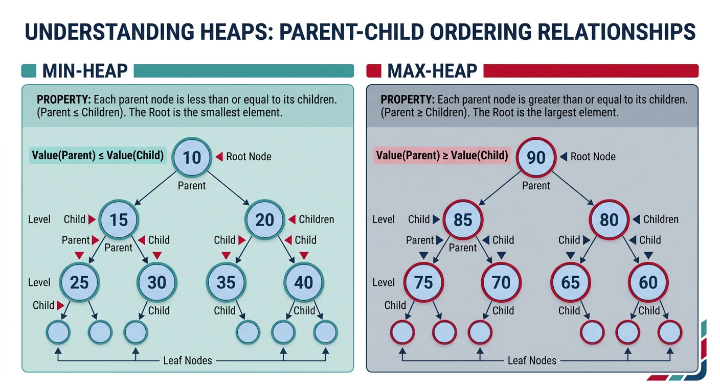
Min heap and max heap side by side showing parent-child ordering relationships — Min heap vs max heap: in a min heap the parent is always smaller than children, in a max heap the parent is always larger

Mental Model: The Heap

Problem it solves: Repeatedly extract the minimum (or maximum) element efficiently. Heaps give \(O(\log n)\) insert and \(O(\log n)\) extract-min — far faster than \(O(n)\) linear scan, with \(O(1)\) peek.

When NOT to use: When you need arbitrary element access or full sorted order — a heap only guarantees fast access to the root. Use a sorted array or BST for full ordering.

Common misconception: "A heap is sorted." It is NOT. Heap order only guarantees parent ≤ children (min-heap) — siblings have no ordering relationship. Heap order ≠ sorted order.

Interview lens: The pattern is: "find or maintain K elements" = heap. Top-K largest, K closest points, K-th smallest, sliding window median, merge K sorted lists — all are heap problems.

Production lens: OS schedulers use priority queues (nice values). Dijkstra's and A* pathfinding are heap-powered. Event-driven simulations process the next-soonest event by always pulling from a min-heap.

                            Heap Structural Properties
                            Max Heap: Parent ≥ Children (root is maximum)
Min Heap: Parent ≤ Children (root is minimum)
Complete Binary Tree: All levels filled except possibly last, filled left to right
Array Representation: For index i: parent = (i-1)//2, left = 2i+1, right = 2i+2

                        

Heap Implementation from Scratch

class MinHeap:
    """
    Min Heap implementation using array
    Root is always the minimum element
    """
    def __init__(self):
        self.heap = []
    
    def parent(self, i):
        return (i - 1) // 2
    
    def left_child(self, i):
        return 2 * i + 1
    
    def right_child(self, i):
        return 2 * i + 2
    
    def swap(self, i, j):
        self.heap[i], self.heap[j] = self.heap[j], self.heap[i]
    
    def insert(self, val):
        """Insert value and maintain heap property - O(log n)"""
        self.heap.append(val)
        self._heapify_up(len(self.heap) - 1)
    
    def _heapify_up(self, i):
        """Bubble up to restore heap property"""
        while i > 0 and self.heap[self.parent(i)] > self.heap[i]:
            self.swap(i, self.parent(i))
            i = self.parent(i)
    
    def extract_min(self):
        """Remove and return minimum element - O(log n)"""
        if not self.heap:
            return None
        
        if len(self.heap) == 1:
            return self.heap.pop()
        
        min_val = self.heap[0]
        self.heap[0] = self.heap.pop()  # Move last to root
        self._heapify_down(0)
        
        return min_val
    
    def _heapify_down(self, i):
        """Bubble down to restore heap property"""
        smallest = i
        left = self.left_child(i)
        right = self.right_child(i)
        
        if left < len(self.heap) and self.heap[left] < self.heap[smallest]:
            smallest = left
        
        if right < len(self.heap) and self.heap[right] < self.heap[smallest]:
            smallest = right
        
        if smallest != i:
            self.swap(i, smallest)
            self._heapify_down(smallest)
    
    def peek(self):
        """Return minimum without removing - O(1)"""
        return self.heap[0] if self.heap else None
    
    def size(self):
        return len(self.heap)

# Example usage
heap = MinHeap()
for val in [5, 3, 8, 1, 2, 9, 4]:
    heap.insert(val)
    print(f"Inserted {val}, heap: {heap.heap}")

print("\nExtracting in sorted order:")
while heap.size() > 0:
    print(heap.extract_min(), end=" ")

// Min Heap Implementation
#include <iostream>
#include <vector>

class MinHeap {
private:
    std::vector<int> heap;
    
    int parent(int i) { return (i - 1) / 2; }
    int left(int i) { return 2 * i + 1; }
    int right(int i) { return 2 * i + 2; }
    
    void heapifyUp(int i) {
        while (i > 0 && heap[parent(i)] > heap[i]) {
            std::swap(heap[i], heap[parent(i)]);
            i = parent(i);
        }
    }
    
    void heapifyDown(int i) {
        int smallest = i;
        int l = left(i), r = right(i);
        
        if (l < heap.size() && heap[l] < heap[smallest]) smallest = l;
        if (r < heap.size() && heap[r] < heap[smallest]) smallest = r;
        
        if (smallest != i) {
            std::swap(heap[i], heap[smallest]);
            heapifyDown(smallest);
        }
    }
    
public:
    void insert(int val) {
        heap.push_back(val);
        heapifyUp(heap.size() - 1);
    }
    
    int extractMin() {
        if (heap.empty()) return -1;
        int minVal = heap[0];
        heap[0] = heap.back();
        heap.pop_back();
        if (!heap.empty()) heapifyDown(0);
        return minVal;
    }
    
    int peek() { return heap.empty() ? -1 : heap[0]; }
    int size() { return heap.size(); }
};

// Min Heap Implementation
import java.util.*;

class MinHeap {
    private List<Integer> heap = new ArrayList<>();
    
    private int parent(int i) { return (i - 1) / 2; }
    private int left(int i) { return 2 * i + 1; }
    private int right(int i) { return 2 * i + 2; }
    
    private void swap(int i, int j) {
        int temp = heap.get(i);
        heap.set(i, heap.get(j));
        heap.set(j, temp);
    }
    
    private void heapifyUp(int i) {
        while (i > 0 && heap.get(parent(i)) > heap.get(i)) {
            swap(i, parent(i));
            i = parent(i);
        }
    }
    
    private void heapifyDown(int i) {
        int smallest = i;
        int l = left(i), r = right(i);
        
        if (l < heap.size() && heap.get(l) < heap.get(smallest)) smallest = l;
        if (r < heap.size() && heap.get(r) < heap.get(smallest)) smallest = r;
        
        if (smallest != i) {
            swap(i, smallest);
            heapifyDown(smallest);
        }
    }
    
    public void insert(int val) {
        heap.add(val);
        heapifyUp(heap.size() - 1);
    }
    
    public int extractMin() {
        if (heap.isEmpty()) return -1;
        int minVal = heap.get(0);
        heap.set(0, heap.get(heap.size() - 1));
        heap.remove(heap.size() - 1);
        if (!heap.isEmpty()) heapifyDown(0);
        return minVal;
    }
    
    public int peek() { return heap.isEmpty() ? -1 : heap.get(0); }
    public int size() { return heap.size(); }
}

Heap Operations

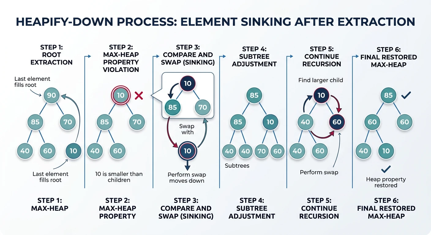
Heapify-down process showing element sinking to correct position after extraction — Heapify-down (sift-down) operation: element at root sinks by swapping with the smaller child until heap property is restored

Heapify-Down (Sift-Down) Decision Flow

                            flowchart TD
                                A(["Extract root (min)"]) --> B["Move last element to root\nheap.size -= 1"]
                                B --> C{"Has children?"}
                                C -->|"No"| G["Heap property restored ✓"]
                                C -->|"Yes"| D["Find smaller child"]
                                D --> E{"Current node >\nsmaller child?"}
                                E -->|"No"| G
                                E -->|"Yes"| F["Swap current with smaller child"]
                                F --> C

Build Heap (Heapify)

Building a heap from an unsorted array seems like it should take \(O(n \log n)\) — insert each element one at a time. But the bottom-up heapify approach is faster: start from the last non-leaf node and sift-down each node. Why \(O(n)\) instead of \(O(n \log n)\)? Most nodes are near the bottom and sift-down very little. Mathematically: half the nodes are leaves (sift 0), a quarter sift 1 level, an eighth sift 2 levels... the sum converges to \(O(n)\).

Analogy: Imagine organizing a company hierarchy from the bottom up — managers at the lowest level check only one report, mid-level managers check two levels, and only the CEO checks the full depth. The total work is dominated by the many small checks at the bottom, not the few expensive ones at the top.

def build_min_heap(arr):
    """
    Build min heap from array in-place
    Time: O(n) - not O(n log n)!
    """
    n = len(arr)
    
    # Start from last non-leaf node and heapify down
    # Last non-leaf node is at index (n // 2) - 1
    for i in range(n // 2 - 1, -1, -1):
        heapify_down(arr, n, i)
    
    return arr

def heapify_down(arr, n, i):
    """Heapify down for min heap"""
    smallest = i
    left = 2 * i + 1
    right = 2 * i + 2
    
    if left < n and arr[left] < arr[smallest]:
        smallest = left
    
    if right < n and arr[right] < arr[smallest]:
        smallest = right
    
    if smallest != i:
        arr[i], arr[smallest] = arr[smallest], arr[i]
        heapify_down(arr, n, smallest)

def build_max_heap(arr):
    """Build max heap from array in-place"""
    n = len(arr)
    
    for i in range(n // 2 - 1, -1, -1):
        max_heapify_down(arr, n, i)
    
    return arr

def max_heapify_down(arr, n, i):
    """Heapify down for max heap"""
    largest = i
    left = 2 * i + 1
    right = 2 * i + 2
    
    if left < n and arr[left] > arr[largest]:
        largest = left
    
    if right < n and arr[right] > arr[largest]:
        largest = right
    
    if largest != i:
        arr[i], arr[largest] = arr[largest], arr[i]
        max_heapify_down(arr, n, largest)

# Example
arr = [4, 10, 3, 5, 1, 8, 7]
print("Original:", arr)

min_heap = build_min_heap(arr.copy())
print("Min heap:", min_heap)

max_heap = build_max_heap(arr.copy())
print("Max heap:", max_heap)

// Build Min/Max Heap in O(n)
#include <iostream>
#include <vector>
#include <algorithm>

void heapifyDownMin(std::vector<int>& arr, int n, int i) {
    int smallest = i;
    int left = 2 * i + 1, right = 2 * i + 2;
    
    if (left < n && arr[left] < arr[smallest]) smallest = left;
    if (right < n && arr[right] < arr[smallest]) smallest = right;
    
    if (smallest != i) {
        std::swap(arr[i], arr[smallest]);
        heapifyDownMin(arr, n, smallest);
    }
}

void heapifyDownMax(std::vector<int>& arr, int n, int i) {
    int largest = i;
    int left = 2 * i + 1, right = 2 * i + 2;
    
    if (left < n && arr[left] > arr[largest]) largest = left;
    if (right < n && arr[right] > arr[largest]) largest = right;
    
    if (largest != i) {
        std::swap(arr[i], arr[largest]);
        heapifyDownMax(arr, n, largest);
    }
}

void buildMinHeap(std::vector<int>& arr) {
    int n = arr.size();
    for (int i = n / 2 - 1; i >= 0; i--)
        heapifyDownMin(arr, n, i);
}

void buildMaxHeap(std::vector<int>& arr) {
    int n = arr.size();
    for (int i = n / 2 - 1; i >= 0; i--)
        heapifyDownMax(arr, n, i);
}

// Also available: std::make_heap (max heap by default)
// std::make_heap(arr.begin(), arr.end());  // Max heap
// std::make_heap(arr.begin(), arr.end(), std::greater<int>());  // Min heap

// Build Min/Max Heap in O(n)
import java.util.*;

class HeapBuilder {
    private static void heapifyDownMin(int[] arr, int n, int i) {
        int smallest = i;
        int left = 2 * i + 1, right = 2 * i + 2;
        
        if (left < n && arr[left] < arr[smallest]) smallest = left;
        if (right < n && arr[right] < arr[smallest]) smallest = right;
        
        if (smallest != i) {
            int temp = arr[i]; arr[i] = arr[smallest]; arr[smallest] = temp;
            heapifyDownMin(arr, n, smallest);
        }
    }
    
    private static void heapifyDownMax(int[] arr, int n, int i) {
        int largest = i;
        int left = 2 * i + 1, right = 2 * i + 2;
        
        if (left < n && arr[left] > arr[largest]) largest = left;
        if (right < n && arr[right] > arr[largest]) largest = right;
        
        if (largest != i) {
            int temp = arr[i]; arr[i] = arr[largest]; arr[largest] = temp;
            heapifyDownMax(arr, n, largest);
        }
    }
    
    public static void buildMinHeap(int[] arr) {
        int n = arr.length;
        for (int i = n / 2 - 1; i >= 0; i--)
            heapifyDownMin(arr, n, i);
    }
    
    public static void buildMaxHeap(int[] arr) {
        int n = arr.length;
        for (int i = n / 2 - 1; i >= 0; i--)
            heapifyDownMax(arr, n, i);
    }
}

// Also available: PriorityQueue
// PriorityQueue<Integer> minHeap = new PriorityQueue<>();
// PriorityQueue<Integer> maxHeap = new PriorityQueue<>(Collections.reverseOrder());

Extract-Min + Heapify-Down — Step-Through

Correct position Being compared Violates heap order Removed

Initial Min-Heap

Root = 1 is the minimum. Click Next to step through the extract-min + heapify-down process.

heap size = 7 Step 1 / 5

Time Complexity Analysis

Operation	Time	Notes
Insert	\(O(\log n)\)	Heapify up
Extract Min/Max	\(O(\log n)\)	Heapify down
Peek	\(O(1)\)	Return root
Build Heap	\(O(n)\)	Not \(O(n \log n)\)!
Heap Sort	\(O(n \log n)\)	Build + n extractions

Python heapq Module

Python's built-in heapq module provides a min-heap backed by a regular list. There is no max-heap variant — to simulate one, negate values on insert and negate again on extraction. The module offers \(O(\log n)\) push/pop and a powerful \(O(n)\) heapify() that converts any list into a valid heap in-place. For interview coding, mastering heapq lets you solve priority queue problems in 3-5 lines instead of implementing from scratch.

                            Key heapq Functions
                            heapq.heappush(heap, item) — push item maintaining heap invariant, \(O(\log n)\)
heapq.heappop(heap) — pop and return smallest, \(O(\log n)\)
heapq.heapify(list) — transform list into heap in-place, \(O(n)\)
heapq.nlargest(k, iterable) — return k largest elements, \(O(n \log k)\)
heapq.heappushpop(heap, item) — push then pop in one operation (faster than separate calls)

                        

import heapq

# Python heapq implements MIN HEAP only
# For max heap, negate values

# Basic operations
heap = []
heapq.heappush(heap, 3)
heapq.heappush(heap, 1)
heapq.heappush(heap, 4)
heapq.heappush(heap, 1)
heapq.heappush(heap, 5)

print("Heap:", heap)  # [1, 1, 4, 3, 5]
print("Min:", heap[0])  # 1 (peek without removing)

# Extract minimum
print("Pop:", heapq.heappop(heap))  # 1
print("After pop:", heap)  # [1, 3, 4, 5]

// C++ priority_queue (Max heap by default)
#include <iostream>
#include <queue>
#include <vector>

int main() {
    // Min heap using greater comparator
    std::priority_queue<int, std::vector<int>, std::greater<int>> minHeap;
    
    minHeap.push(3);
    minHeap.push(1);
    minHeap.push(4);
    minHeap.push(1);
    minHeap.push(5);
    
    std::cout << "Min: " << minHeap.top() << std::endl;  // 1
    
    minHeap.pop();
    std::cout << "After pop, Min: " << minHeap.top() << std::endl;  // 1
    
    return 0;
}

// Java PriorityQueue (Min heap by default)
import java.util.*;

public class HeapDemo {
    public static void main(String[] args) {
        // Min heap (default)
        PriorityQueue<Integer> minHeap = new PriorityQueue<>();
        
        minHeap.add(3);
        minHeap.add(1);
        minHeap.add(4);
        minHeap.add(1);
        minHeap.add(5);
        
        System.out.println("Heap: " + minHeap);  // [1, 1, 4, 3, 5]
        System.out.println("Min: " + minHeap.peek());  // 1
        
        System.out.println("Pop: " + minHeap.poll());  // 1
        System.out.println("After pop: " + minHeap);
    }
}

import heapq

# heapify - Convert list to heap in-place O(n)
arr = [5, 7, 9, 1, 3]
heapq.heapify(arr)
print("Heapified:", arr)  # [1, 3, 9, 7, 5]

# nlargest and nsmallest - O(n log k)
nums = [3, 1, 4, 1, 5, 9, 2, 6, 5, 3]
print("3 largest:", heapq.nlargest(3, nums))   # [9, 6, 5]
print("3 smallest:", heapq.nsmallest(3, nums))  # [1, 1, 2]

# With key function
people = [('Alice', 30), ('Bob', 25), ('Charlie', 35)]
print("Oldest:", heapq.nlargest(1, people, key=lambda x: x[1]))

import heapq

# Max Heap using negative values
max_heap = []
values = [3, 1, 4, 1, 5, 9]

for val in values:
    heapq.heappush(max_heap, -val)  # Negate to simulate max heap

print("Max heap (negated):", max_heap)

# Extract max
max_val = -heapq.heappop(max_heap)
print("Maximum:", max_val)  # 9

import heapq

# Priority Queue with tuples (priority, item)
# Lower priority value = higher priority
pq = []
heapq.heappush(pq, (2, "task B"))
heapq.heappush(pq, (1, "task A"))
heapq.heappush(pq, (3, "task C"))

print("Processing order:")
while pq:
    priority, task = heapq.heappop(pq)
    print(f"  {task} (priority {priority})")

Heap Applications

Heaps shine in problems that repeatedly ask for the extreme element (smallest/largest) from a changing collection. The universal interview pattern: "find K-th / top-K / K closest" — maintain a heap of size K, and every element beyond K either enters (bumping one out) or is discarded. This gives \(O(n \log k)\) instead of \(O(n \log n)\) sorting.

Kth Largest Element

Maintain a min-heap of size K. As you scan the array, push each element; if the heap exceeds size K, pop the smallest (it can't be in the top-K). After processing all elements, the heap root is the K-th largest. This is \(O(n \log k)\) time, \(O(k)\) space — much better than \(O(n \log n)\) full sort when \(k \ll n\). The alternative Quick-Select gives \(O(n)\) average but \(O(n^2)\) worst case.

import heapq

def find_kth_largest(nums, k):
    """
    LeetCode 215: Kth Largest Element in an Array
    Use min heap of size k
    Time: O(n log k), Space: O(k)
    """
    # Maintain min heap of k largest elements
    min_heap = []
    
    for num in nums:
        heapq.heappush(min_heap, num)
        
        # Keep only k elements
        if len(min_heap) > k:
            heapq.heappop(min_heap)
    
    # Root is kth largest
    return min_heap[0]

def find_kth_largest_quick(nums, k):
    """
    Alternative using nlargest - cleaner
    Time: O(n log k)
    """
    return heapq.nlargest(k, nums)[-1]

# Example
nums = [3, 2, 1, 5, 6, 4]
k = 2
print(f"Array: {nums}")
print(f"{k}th largest: {find_kth_largest(nums, k)}")  # 5

nums = [3, 2, 3, 1, 2, 4, 5, 5, 6]
k = 4
print(f"{k}th largest: {find_kth_largest(nums, k)}")  # 4

// LeetCode 215 - Kth Largest Element
// Time: O(n log k), Space: O(k)
#include <vector>
#include <queue>

class Solution {
public:
    int findKthLargest(std::vector<int>& nums, int k) {
        // Min heap of size k
        std::priority_queue<int, std::vector<int>, std::greater<int>> minHeap;
        
        for (int num : nums) {
            minHeap.push(num);
            if (minHeap.size() > k) {
                minHeap.pop();
            }
        }
        
        return minHeap.top();
    }
};

// LeetCode 215 - Kth Largest Element
// Time: O(n log k), Space: O(k)
import java.util.*;

class Solution {
    public int findKthLargest(int[] nums, int k) {
        // Min heap of size k
        PriorityQueue<Integer> minHeap = new PriorityQueue<>();
        
        for (int num : nums) {
            minHeap.add(num);
            if (minHeap.size() > k) {
                minHeap.poll();
            }
        }
        
        return minHeap.peek();
    }
}

Top K Frequent Elements

A two-phase problem: first count frequencies using a hash map (\(O(n)\)), then find the K most frequent. A min-heap of size K holding (frequency, element) pairs does this in \(O(n \log k)\). Alternative: bucket sort by frequency — create buckets indexed 1..n where bucket[f] contains all elements with frequency f, then collect from highest bucket down. This gives \(O(n)\) but uses more space.

import heapq
from collections import Counter

def top_k_frequent(nums, k):
    """
    LeetCode 347: Top K Frequent Elements
    Time: O(n log k), Space: O(n)
    """
    # Count frequencies
    freq = Counter(nums)
    
    # Use min heap of size k
    # Store (frequency, element)
    min_heap = []
    
    for num, count in freq.items():
        heapq.heappush(min_heap, (count, num))
        
        if len(min_heap) > k:
            heapq.heappop(min_heap)
    
    # Extract elements
    return [item[1] for item in min_heap]

# Example
nums = [1, 1, 1, 2, 2, 3]
k = 2
print(f"Top {k} frequent:", top_k_frequent(nums, k))  # [2, 1]

nums = [1]
k = 1
print(f"Top {k} frequent:", top_k_frequent(nums, k))  # [1]

// LeetCode 347 - Top K Frequent Elements
// Time: O(n log k), Space: O(n)
#include <vector>
#include <queue>
#include <unordered_map>

class Solution {
public:
    std::vector<int> topKFrequent(std::vector<int>& nums, int k) {
        // Count frequencies
        std::unordered_map<int, int> freq;
        for (int num : nums) freq[num]++;
        
        // Min heap of (frequency, element)
        auto cmp = [](std::pair<int,int>& a, std::pair<int,int>& b) {
            return a.first > b.first;
        };
        std::priority_queue<std::pair<int,int>, std::vector<std::pair<int,int>>, decltype(cmp)> minHeap(cmp);
        
        for (auto& [num, count] : freq) {
            minHeap.push({count, num});
            if (minHeap.size() > k) minHeap.pop();
        }
        
        std::vector<int> result;
        while (!minHeap.empty()) {
            result.push_back(minHeap.top().second);
            minHeap.pop();
        }
        return result;
    }
};

// LeetCode 347 - Top K Frequent Elements
// Time: O(n log k), Space: O(n)
import java.util.*;

class Solution {
    public int[] topKFrequent(int[] nums, int k) {
        // Count frequencies
        Map<Integer, Integer> freq = new HashMap<>();
        for (int num : nums) freq.put(num, freq.getOrDefault(num, 0) + 1);
        
        // Min heap by frequency
        PriorityQueue<int[]> minHeap = new PriorityQueue<>((a, b) -> a[0] - b[0]);
        
        for (Map.Entry<Integer, Integer> entry : freq.entrySet()) {
            minHeap.add(new int[]{entry.getValue(), entry.getKey()});
            if (minHeap.size() > k) minHeap.poll();
        }
        
        int[] result = new int[k];
        for (int i = 0; i < k; i++) {
            result[i] = minHeap.poll()[1];
        }
        return result;
    }
}

Merge K Sorted Lists

Given K sorted linked lists, merge them into one sorted list. The naive approach compares all K heads each step (\(O(nk)\) total). A min-heap of size K holding the current head of each list reduces each extraction to \(O(\log k)\), giving \(O(n \log k)\) total where n is the total number of nodes. This is a fundamental pattern in external sorting — when data doesn't fit in memory, sort chunks individually, then K-way merge the sorted chunks using a heap.

import heapq

class ListNode:
    def __init__(self, val=0, next=None):
        self.val = val
        self.next = next

def merge_k_lists(lists):
    """
    LeetCode 23: Merge k Sorted Lists
    Time: O(n log k) where n = total nodes, k = number of lists
    Space: O(k) for heap
    """
    # Min heap: (value, index, node)
    # Index is for tie-breaking (nodes aren't comparable)
    heap = []
    
    # Initialize heap with first node of each list
    for i, node in enumerate(lists):
        if node:
            heapq.heappush(heap, (node.val, i, node))
    
    # Dummy head for result
    dummy = ListNode(0)
    current = dummy
    
    while heap:
        val, idx, node = heapq.heappop(heap)
        
        # Add to result
        current.next = node
        current = current.next
        
        # Push next node from same list
        if node.next:
            heapq.heappush(heap, (node.next.val, idx, node.next))
    
    return dummy.next

# Helper to create list from array
def create_list(arr):
    dummy = ListNode(0)
    curr = dummy
    for val in arr:
        curr.next = ListNode(val)
        curr = curr.next
    return dummy.next

def list_to_array(head):
    result = []
    while head:
        result.append(head.val)
        head = head.next
    return result

# Example
lists = [
    create_list([1, 4, 5]),
    create_list([1, 3, 4]),
    create_list([2, 6])
]

merged = merge_k_lists(lists)
print("Merged:", list_to_array(merged))  # [1, 1, 2, 3, 4, 4, 5, 6]

// LeetCode 23 - Merge K Sorted Lists
// Time: O(n log k), Space: O(k)
#include <vector>
#include <queue>

struct ListNode {
    int val;
    ListNode* next;
    ListNode(int x) : val(x), next(nullptr) {}
};

class Solution {
public:
    ListNode* mergeKLists(std::vector<ListNode*>& lists) {
        auto cmp = [](ListNode* a, ListNode* b) { return a->val > b->val; };
        std::priority_queue<ListNode*, std::vector<ListNode*>, decltype(cmp)> minHeap(cmp);
        
        for (ListNode* node : lists) {
            if (node) minHeap.push(node);
        }
        
        ListNode dummy(0);
        ListNode* current = &dummy;
        
        while (!minHeap.empty()) {
            ListNode* node = minHeap.top(); minHeap.pop();
            current->next = node;
            current = current->next;
            if (node->next) minHeap.push(node->next);
        }
        
        return dummy.next;
    }
};

// LeetCode 23 - Merge K Sorted Lists
// Time: O(n log k), Space: O(k)
import java.util.*;

class Solution {
    public ListNode mergeKLists(ListNode[] lists) {
        PriorityQueue<ListNode> minHeap = new PriorityQueue<>((a, b) -> a.val - b.val);
        
        for (ListNode node : lists) {
            if (node != null) minHeap.add(node);
        }
        
        ListNode dummy = new ListNode(0);
        ListNode current = dummy;
        
        while (!minHeap.isEmpty()) {
            ListNode node = minHeap.poll();
            current.next = node;
            current = current.next;
            if (node.next != null) minHeap.add(node.next);
        }
        
        return dummy.next;
    }
}

Sorting Algorithms Overview

Sorting Algorithms Comparison

Algorithm	Best	Average	Worst	Space	Stable
Merge Sort	\(O(n \log n)\)	\(O(n \log n)\)	\(O(n \log n)\)	\(O(n)\)	Yes
Quick Sort	\(O(n \log n)\)	\(O(n \log n)\)	\(O(n^{2})\)	\(O(\log n)\)	No
Heap Sort	\(O(n \log n)\)	\(O(n \log n)\)	\(O(n \log n)\)	\(O(1)\)	No
Counting Sort	O(n+k)	O(n+k)	O(n+k)	\(O(k)\)	Yes
Radix Sort	O(nk)	O(nk)	O(nk)	O(n+k)	Yes
Bubble Sort	\(O(n)\)	\(O(n^{2})\)	\(O(n^{2})\)	\(O(1)\)	Yes
Insertion Sort	\(O(n)\)	\(O(n^{2})\)	\(O(n^{2})\)	\(O(1)\)	Yes

Sorting Complexity — Visual Comparison

Relative “cost” per algorithm at n = 10,000 (normalised to Merge Sort = 1.0). Lower is better for time; hover for space and stability.

Merge Sort

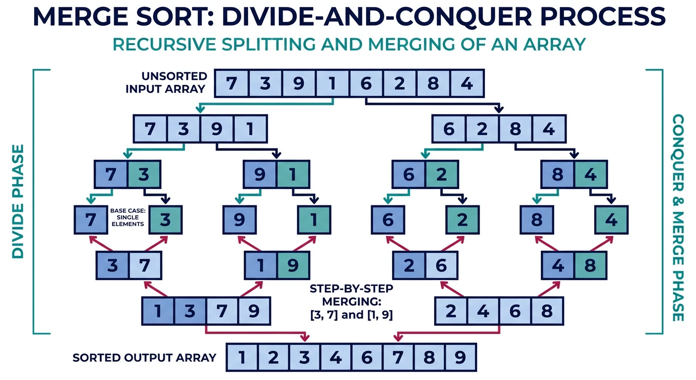
Merge Sort is the quintessential divide-and-conquer algorithm. It splits the array in half, recursively sorts each half, then merges the two sorted halves in linear time. The genius is that merging two sorted arrays is trivial — just compare the front elements and take the smaller. This guarantees \(O(n \log n)\) in all cases (best, average, worst) — no degenerate inputs exist.

Merge Sort: Tradeoffs

Strengths: Guaranteed \(O(n \log n)\), stable (preserves relative order of equal elements), parallelizable (both halves can be sorted independently), and the go-to for linked list sorting (no random access needed).

Weaknesses: \(O(n)\) extra space for the auxiliary array. For in-memory sorting of arrays, Quick Sort is often faster in practice due to better cache locality.

Real-world usage: Python's sorted() and Java's Arrays.sort() for objects use Timsort — a hybrid of Merge Sort and Insertion Sort that exploits existing order ("runs") in real data.

Merge sort divide-and-conquer process showing recursive splitting and merging of array — Merge sort: recursively divide array into halves, sort each half, then merge sorted subarrays back together

def merge_sort(arr):
    """
    Merge Sort - Divide and Conquer
    Time: O(n log n), Space: O(n)
    Stable: Yes
    """
    if len(arr) <= 1:
        return arr
    
    # Divide
    mid = len(arr) // 2
    left = merge_sort(arr[:mid])
    right = merge_sort(arr[mid:])
    
    # Conquer (merge)
    return merge(left, right)

def merge(left, right):
    """Merge two sorted arrays"""
    result = []
    i = j = 0
    
    while i < len(left) and j < len(right):
        if left[i] <= right[j]:  # <= for stability
            result.append(left[i])
            i += 1
        else:
            result.append(right[j])
            j += 1
    
    # Add remaining elements
    result.extend(left[i:])
    result.extend(right[j:])
    
    return result

# Example
arr = [38, 27, 43, 3, 9, 82, 10]
print("Original:", arr)
print("Sorted:", merge_sort(arr))

// Merge Sort - Divide and Conquer
// Time: O(n log n), Space: O(n), Stable: Yes
#include <vector>

class MergeSort {
private:
    static std::vector<int> merge(std::vector<int>& left, std::vector<int>& right) {
        std::vector<int> result;
        int i = 0, j = 0;
        
        while (i < left.size() && j < right.size()) {
            if (left[i] <= right[j]) result.push_back(left[i++]);
            else result.push_back(right[j++]);
        }
        
        while (i < left.size()) result.push_back(left[i++]);
        while (j < right.size()) result.push_back(right[j++]);
        
        return result;
    }
    
public:
    static std::vector<int> sort(std::vector<int> arr) {
        if (arr.size() <= 1) return arr;
        
        int mid = arr.size() / 2;
        std::vector<int> left(arr.begin(), arr.begin() + mid);
        std::vector<int> right(arr.begin() + mid, arr.end());
        
        left = sort(left);
        right = sort(right);
        
        return merge(left, right);
    }
};

// Also available: std::sort (introsort) and std::stable_sort (merge sort)

// Merge Sort - Divide and Conquer
// Time: O(n log n), Space: O(n), Stable: Yes
import java.util.*;

class MergeSort {
    public static int[] sort(int[] arr) {
        if (arr.length <= 1) return arr;
        
        int mid = arr.length / 2;
        int[] left = sort(Arrays.copyOfRange(arr, 0, mid));
        int[] right = sort(Arrays.copyOfRange(arr, mid, arr.length));
        
        return merge(left, right);
    }
    
    private static int[] merge(int[] left, int[] right) {
        int[] result = new int[left.length + right.length];
        int i = 0, j = 0, k = 0;
        
        while (i < left.length && j < right.length) {
            if (left[i] <= right[j]) result[k++] = left[i++];
            else result[k++] = right[j++];
        }
        
        while (i < left.length) result[k++] = left[i++];
        while (j < right.length) result[k++] = right[j++];
        
        return result;
    }
}

// Also available: Arrays.sort() uses dual-pivot quicksort for primitives,
// merge sort for objects (stable)

def merge_sort_inplace(arr, left, right):
    """
    Merge Sort - In-place variant (still O(n) space for merge)
    Useful for linked lists where O(1) space is achievable
    """
    if left < right:
        mid = (left + right) // 2
        
        merge_sort_inplace(arr, left, mid)
        merge_sort_inplace(arr, mid + 1, right)
        merge_inplace(arr, left, mid, right)

def merge_inplace(arr, left, mid, right):
    """Merge two sorted subarrays using auxiliary space"""
    # Create temp arrays
    left_arr = arr[left:mid + 1]
    right_arr = arr[mid + 1:right + 1]
    
    i = j = 0
    k = left
    
    while i < len(left_arr) and j < len(right_arr):
        if left_arr[i] <= right_arr[j]:
            arr[k] = left_arr[i]
            i += 1
        else:
            arr[k] = right_arr[j]
            j += 1
        k += 1
    
    while i < len(left_arr):
        arr[k] = left_arr[i]
        i += 1
        k += 1
    
    while j < len(right_arr):
        arr[k] = right_arr[j]
        j += 1
        k += 1

# Example
arr = [12, 11, 13, 5, 6, 7]
print("Original:", arr)
merge_sort_inplace(arr, 0, len(arr) - 1)
print("Sorted:", arr)

// Merge Sort - In-place variant
#include <vector>
#include <algorithm>

class MergeSortInplace {
private:
    static void merge(std::vector<int>& arr, int left, int mid, int right) {
        std::vector<int> leftArr(arr.begin() + left, arr.begin() + mid + 1);
        std::vector<int> rightArr(arr.begin() + mid + 1, arr.begin() + right + 1);
        
        int i = 0, j = 0, k = left;
        
        while (i < leftArr.size() && j < rightArr.size()) {
            if (leftArr[i] <= rightArr[j]) arr[k++] = leftArr[i++];
            else arr[k++] = rightArr[j++];
        }
        
        while (i < leftArr.size()) arr[k++] = leftArr[i++];
        while (j < rightArr.size()) arr[k++] = rightArr[j++];
    }
    
public:
    static void sort(std::vector<int>& arr, int left, int right) {
        if (left < right) {
            int mid = left + (right - left) / 2;
            sort(arr, left, mid);
            sort(arr, mid + 1, right);
            merge(arr, left, mid, right);
        }
    }
};

// Merge Sort - In-place variant
import java.util.*;

class MergeSortInplace {
    public static void sort(int[] arr, int left, int right) {
        if (left < right) {
            int mid = left + (right - left) / 2;
            sort(arr, left, mid);
            sort(arr, mid + 1, right);
            merge(arr, left, mid, right);
        }
    }
    
    private static void merge(int[] arr, int left, int mid, int right) {
        int[] leftArr = Arrays.copyOfRange(arr, left, mid + 1);
        int[] rightArr = Arrays.copyOfRange(arr, mid + 1, right + 1);
        
        int i = 0, j = 0, k = left;
        
        while (i < leftArr.length && j < rightArr.length) {
            if (leftArr[i] <= rightArr[j]) arr[k++] = leftArr[i++];
            else arr[k++] = rightArr[j++];
        }
        
        while (i < leftArr.length) arr[k++] = leftArr[i++];
        while (j < rightArr.length) arr[k++] = rightArr[j++];
    }
}

Quick Sort

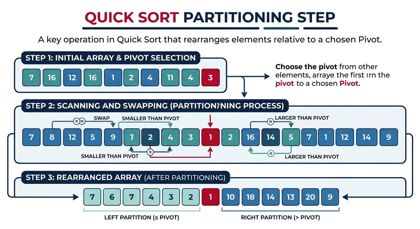
Quick Sort selects a pivot element, then partitions the array: all elements smaller than the pivot go left, all larger go right. Then recursively sort each partition. The key operation is the partition step — done in-place in \(O(n)\) time with a two-pointer technique. Unlike Merge Sort which does work when merging, Quick Sort does work when dividing.

Why is Quick Sort usually faster than Merge Sort? Despite having \(O(n^2)\) worst case, Quick Sort has better cache locality (operates on contiguous memory, no auxiliary array), smaller constant factors, and the worst case is avoidable with randomized pivot selection. In practice, Quick Sort is 2-3× faster than Merge Sort for in-memory arrays.

Avoiding \(O(n^2)\) Worst Case

The worst case occurs when the pivot is always the smallest or largest element (already sorted arrays with naive first/last pivot). Solutions: (1) Random pivot selection, (2) Median-of-three (pick median of first, middle, last), (3) Introsort (switch to Heap Sort if recursion depth exceeds \(2 \log n\) — used by C++ STL). Always use randomized pivots in interviews.

Quick sort partitioning step showing pivot selection and elements rearranged into left and right partitions — Quick sort partitioning: select a pivot, place smaller elements left and larger elements right, then recursively sort each partition

def quick_sort(arr):
    """
    Quick Sort - Simple implementation
    Time: O(n log n) average, O(n²) worst
    Space: O(log n) average for recursion
    """
    if len(arr) <= 1:
        return arr
    
    pivot = arr[len(arr) // 2]  # Middle element as pivot
    
    left = [x for x in arr if x < pivot]
    middle = [x for x in arr if x == pivot]
    right = [x for x in arr if x > pivot]
    
    return quick_sort(left) + middle + quick_sort(right)

# Example
arr = [3, 6, 8, 10, 1, 2, 1]
print("Original:", arr)
print("Sorted:", quick_sort(arr))

// Quick Sort - Simple implementation
// Time: O(n log n) average, O(n²) worst, Space: O(log n)
#include <vector>
#include <algorithm>

class QuickSort {
public:
    static std::vector<int> sort(std::vector<int> arr) {
        if (arr.size() <= 1) return arr;
        
        int pivot = arr[arr.size() / 2];
        std::vector<int> left, middle, right;
        
        for (int x : arr) {
            if (x < pivot) left.push_back(x);
            else if (x == pivot) middle.push_back(x);
            else right.push_back(x);
        }
        
        left = sort(left);
        right = sort(right);
        
        left.insert(left.end(), middle.begin(), middle.end());
        left.insert(left.end(), right.begin(), right.end());
        return left;
    }
};

// Quick Sort - Simple implementation
// Time: O(n log n) average, O(n²) worst, Space: O(log n)
import java.util.*;

class QuickSort {
    public static List<Integer> sort(List<Integer> arr) {
        if (arr.size() <= 1) return new ArrayList<>(arr);
        
        int pivot = arr.get(arr.size() / 2);
        List<Integer> left = new ArrayList<>();
        List<Integer> middle = new ArrayList<>();
        List<Integer> right = new ArrayList<>();
        
        for (int x : arr) {
            if (x < pivot) left.add(x);
            else if (x == pivot) middle.add(x);
            else right.add(x);
        }
        
        List<Integer> result = sort(left);
        result.addAll(middle);
        result.addAll(sort(right));
        return result;
    }
}

def quick_sort_inplace(arr, low, high):
    """
    Quick Sort - In-place with Lomuto partition
    More memory efficient
    """
    if low < high:
        # Partition and get pivot index
        pivot_idx = partition(arr, low, high)
        
        # Recursively sort partitions
        quick_sort_inplace(arr, low, pivot_idx - 1)
        quick_sort_inplace(arr, pivot_idx + 1, high)

def partition(arr, low, high):
    """
    Lomuto partition scheme
    Pivot is last element
    """
    pivot = arr[high]
    i = low - 1  # Index of smaller element
    
    for j in range(low, high):
        if arr[j] <= pivot:
            i += 1
            arr[i], arr[j] = arr[j], arr[i]
    
    # Place pivot in correct position
    arr[i + 1], arr[high] = arr[high], arr[i + 1]
    
    return i + 1

# Example
arr = [10, 7, 8, 9, 1, 5]
print("Original:", arr)
quick_sort_inplace(arr, 0, len(arr) - 1)
print("Sorted:", arr)

// Quick Sort - In-place with Lomuto partition
#include <vector>
#include <algorithm>

class QuickSortInplace {
private:
    static int partition(std::vector<int>& arr, int low, int high) {
        int pivot = arr[high];
        int i = low - 1;
        
        for (int j = low; j < high; j++) {
            if (arr[j] <= pivot) {
                i++;
                std::swap(arr[i], arr[j]);
            }
        }
        std::swap(arr[i + 1], arr[high]);
        return i + 1;
    }
    
public:
    static void sort(std::vector<int>& arr, int low, int high) {
        if (low < high) {
            int pivotIdx = partition(arr, low, high);
            sort(arr, low, pivotIdx - 1);
            sort(arr, pivotIdx + 1, high);
        }
    }
};

// Quick Sort - In-place with Lomuto partition

class QuickSortInplace {
    public static void sort(int[] arr, int low, int high) {
        if (low < high) {
            int pivotIdx = partition(arr, low, high);
            sort(arr, low, pivotIdx - 1);
            sort(arr, pivotIdx + 1, high);
        }
    }
    
    private static int partition(int[] arr, int low, int high) {
        int pivot = arr[high];
        int i = low - 1;
        
        for (int j = low; j < high; j++) {
            if (arr[j] <= pivot) {
                i++;
                int temp = arr[i]; arr[i] = arr[j]; arr[j] = temp;
            }
        }
        int temp = arr[i + 1]; arr[i + 1] = arr[high]; arr[high] = temp;
        return i + 1;
    }
}

import random

def quick_sort_randomized(arr, low, high):
    """
    Randomized Quick Sort
    Avoids O(n²) worst case by random pivot selection
    """
    if low < high:
        pivot_idx = randomized_partition(arr, low, high)
        quick_sort_randomized(arr, low, pivot_idx - 1)
        quick_sort_randomized(arr, pivot_idx + 1, high)

def randomized_partition(arr, low, high):
    """Randomly select pivot and partition"""
    # Random pivot
    rand_idx = random.randint(low, high)
    arr[rand_idx], arr[high] = arr[high], arr[rand_idx]
    
    # Standard partition
    pivot = arr[high]
    i = low - 1
    
    for j in range(low, high):
        if arr[j] <= pivot:
            i += 1
            arr[i], arr[j] = arr[j], arr[i]
    
    arr[i + 1], arr[high] = arr[high], arr[i + 1]
    return i + 1

# Example with already sorted array (worst case for standard quick sort)
arr = [1, 2, 3, 4, 5, 6, 7, 8, 9, 10]
print("Original (sorted):", arr)
quick_sort_randomized(arr, 0, len(arr) - 1)
print("After randomized quick sort:", arr)

// Randomized Quick Sort - Avoids O(n²) worst case
#include <vector>
#include <algorithm>
#include <random>

class RandomizedQuickSort {
private:
    static int randomizedPartition(std::vector<int>& arr, int low, int high) {
        // Random pivot selection
        int randIdx = low + rand() % (high - low + 1);
        std::swap(arr[randIdx], arr[high]);
        
        int pivot = arr[high];
        int i = low - 1;
        
        for (int j = low; j < high; j++) {
            if (arr[j] <= pivot) {
                i++;
                std::swap(arr[i], arr[j]);
            }
        }
        std::swap(arr[i + 1], arr[high]);
        return i + 1;
    }
    
public:
    static void sort(std::vector<int>& arr, int low, int high) {
        if (low < high) {
            int pivotIdx = randomizedPartition(arr, low, high);
            sort(arr, low, pivotIdx - 1);
            sort(arr, pivotIdx + 1, high);
        }
    }
};

// Randomized Quick Sort - Avoids O(n²) worst case
import java.util.*;

class RandomizedQuickSort {
    private static Random rand = new Random();
    
    public static void sort(int[] arr, int low, int high) {
        if (low < high) {
            int pivotIdx = randomizedPartition(arr, low, high);
            sort(arr, low, pivotIdx - 1);
            sort(arr, pivotIdx + 1, high);
        }
    }
    
    private static int randomizedPartition(int[] arr, int low, int high) {
        // Random pivot selection
        int randIdx = low + rand.nextInt(high - low + 1);
        int temp = arr[randIdx]; arr[randIdx] = arr[high]; arr[high] = temp;
        
        int pivot = arr[high];
        int i = low - 1;
        
        for (int j = low; j < high; j++) {
            if (arr[j] <= pivot) {
                i++;
                temp = arr[i]; arr[i] = arr[j]; arr[j] = temp;
            }
        }
        temp = arr[i + 1]; arr[i + 1] = arr[high]; arr[high] = temp;
        return i + 1;
    }
}

Heap Sort

Heap Sort combines the heap's extraction property with in-place sorting. The algorithm has two phases: (1) Build a max-heap from the unsorted array in \(O(n)\) — now the maximum is at index 0. (2) Repeatedly swap the root (maximum) with the last unsorted element, shrink the heap by one, and sift-down to restore the heap property. After \(n-1\) extractions, the array is sorted.

When to choose Heap Sort: It guarantees \(O(n \log n)\) worst case with \(O(1)\) extra space — making it ideal when memory is constrained and worst-case guarantees matter (embedded systems, real-time systems). The tradeoff: it's not stable and has poor cache locality (parent-child jumps in the array are not sequential), making it ~2× slower than Quick Sort in practice for random data.

def heap_sort(arr):
    """
    Heap Sort - In-place sorting using max heap
    Time: O(n log n), Space: O(1)
    Not stable
    """
    n = len(arr)
    
    # Build max heap - O(n)
    for i in range(n // 2 - 1, -1, -1):
        heapify(arr, n, i)
    
    # Extract elements one by one - O(n log n)
    for i in range(n - 1, 0, -1):
        # Move current root (max) to end
        arr[0], arr[i] = arr[i], arr[0]
        
        # Heapify reduced heap
        heapify(arr, i, 0)
    
    return arr

def heapify(arr, n, i):
    """
    Heapify subtree rooted at index i
    n is size of heap
    """
    largest = i
    left = 2 * i + 1
    right = 2 * i + 2
    
    if left < n and arr[left] > arr[largest]:
        largest = left
    
    if right < n and arr[right] > arr[largest]:
        largest = right
    
    if largest != i:
        arr[i], arr[largest] = arr[largest], arr[i]
        heapify(arr, n, largest)

# Example
arr = [12, 11, 13, 5, 6, 7]
print("Original:", arr)
heap_sort(arr)
print("Sorted:", arr)

# Test with larger array
import random
arr = [random.randint(1, 100) for _ in range(15)]
print("\nRandom array:", arr)
heap_sort(arr)
print("Sorted:", arr)

// Heap Sort - In-place using max heap
// Time: O(n log n), Space: O(1), Not stable
#include <vector>
#include <algorithm>

class HeapSort {
private:
    static void heapify(std::vector<int>& arr, int n, int i) {
        int largest = i;
        int left = 2 * i + 1, right = 2 * i + 2;
        
        if (left < n && arr[left] > arr[largest]) largest = left;
        if (right < n && arr[right] > arr[largest]) largest = right;
        
        if (largest != i) {
            std::swap(arr[i], arr[largest]);
            heapify(arr, n, largest);
        }
    }
    
public:
    static void sort(std::vector<int>& arr) {
        int n = arr.size();
        
        // Build max heap
        for (int i = n / 2 - 1; i >= 0; i--)
            heapify(arr, n, i);
        
        // Extract elements one by one
        for (int i = n - 1; i > 0; i--) {
            std::swap(arr[0], arr[i]);
            heapify(arr, i, 0);
        }
    }
};

// Also available: std::sort_heap after std::make_heap

// Heap Sort - In-place using max heap
// Time: O(n log n), Space: O(1), Not stable

class HeapSort {
    public static void sort(int[] arr) {
        int n = arr.length;
        
        // Build max heap
        for (int i = n / 2 - 1; i >= 0; i--)
            heapify(arr, n, i);
        
        // Extract elements one by one
        for (int i = n - 1; i > 0; i--) {
            int temp = arr[0]; arr[0] = arr[i]; arr[i] = temp;
            heapify(arr, i, 0);
        }
    }
    
    private static void heapify(int[] arr, int n, int i) {
        int largest = i;
        int left = 2 * i + 1, right = 2 * i + 2;
        
        if (left < n && arr[left] > arr[largest]) largest = left;
        if (right < n && arr[right] > arr[largest]) largest = right;
        
        if (largest != i) {
            int temp = arr[i]; arr[i] = arr[largest]; arr[largest] = temp;
            heapify(arr, n, largest);
        }
    }
}

Hash Tables

A Hash Table (HashMap/Dictionary) is arguably the most important data structure in software engineering. It provides \(O(1)\) average-case lookup, insert, and delete by using a hash function to map keys directly to array indices. Think of it like a library's card catalog: instead of searching every shelf, you compute exactly which shelf a book belongs on.

How it works: (1) Compute hash(key) % array_size to get a bucket index. (2) Store the key-value pair at that index. (3) On lookup, compute the same hash to find the bucket directly. The magic: going from \(O(n)\) linear search to \(O(1)\) constant-time access by trading space for speed.

Real-world ubiquity: Python dict, JavaScript objects, Java HashMap, C++ unordered_map, database indexes, caching layers (Redis/Memcached), DNS resolution, compiler symbol tables — all powered by hashing. In interviews, if you need to check "have I seen this before?" or "count occurrences" — the answer is almost always a hash map.

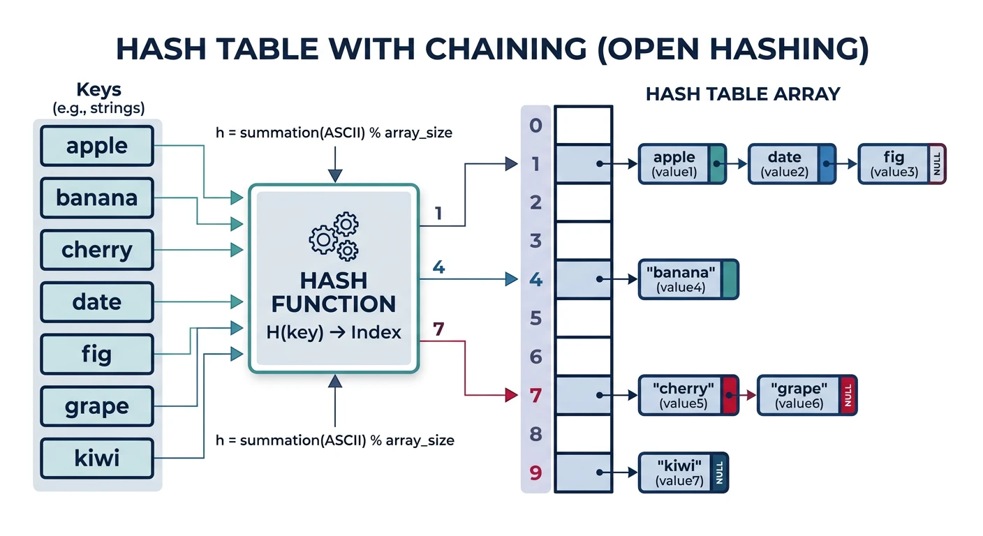
Hash table showing keys mapped through hash function to array bucket indices with chaining — Hash table architecture: keys are mapped through a hash function to bucket indices, with chaining used for collision resolution

                            Hash Table Concepts
                            Hash Function: Maps keys to array indices
Collision: When two keys hash to same index
Load Factor: n/m (items/buckets) - typically keep < 0.75
Rehashing: Resize and rehash when load factor exceeds threshold

                        

class HashTable:
    """
    Hash Table with chaining for collision resolution
    """
    def __init__(self, size=10):
        self.size = size
        self.buckets = [[] for _ in range(size)]
        self.count = 0
    
    def _hash(self, key):
        """Simple hash function"""
        return hash(key) % self.size
    
    def put(self, key, value):
        """Insert or update key-value pair - O(1) average"""
        index = self._hash(key)
        
        # Check if key exists, update if so
        for i, (k, v) in enumerate(self.buckets[index]):
            if k == key:
                self.buckets[index][i] = (key, value)
                return
        
        # Add new key-value pair
        self.buckets[index].append((key, value))
        self.count += 1
        
        # Rehash if load factor > 0.75
        if self.count / self.size > 0.75:
            self._rehash()
    
    def get(self, key):
        """Get value by key - O(1) average"""
        index = self._hash(key)
        
        for k, v in self.buckets[index]:
            if k == key:
                return v
        
        return None  # Key not found
    
    def remove(self, key):
        """Remove key-value pair - O(1) average"""
        index = self._hash(key)
        
        for i, (k, v) in enumerate(self.buckets[index]):
            if k == key:
                del self.buckets[index][i]
                self.count -= 1
                return True
        
        return False  # Key not found
    
    def _rehash(self):
        """Double size and rehash all elements"""
        old_buckets = self.buckets
        self.size *= 2
        self.buckets = [[] for _ in range(self.size)]
        self.count = 0
        
        for bucket in old_buckets:
            for key, value in bucket:
                self.put(key, value)
    
    def __str__(self):
        items = []
        for bucket in self.buckets:
            for k, v in bucket:
                items.append(f"{k}: {v}")
        return "{" + ", ".join(items) + "}"

# Example usage
ht = HashTable()
ht.put("apple", 5)
ht.put("banana", 3)
ht.put("cherry", 8)
ht.put("date", 2)

print("Hash table:", ht)
print("Get 'banana':", ht.get("banana"))

ht.put("banana", 10)  # Update
print("After update:", ht.get("banana"))

ht.remove("cherry")
print("After remove:", ht)

// Hash Table with Chaining (Separate Chaining)
#include <vector>
#include <list>
#include <optional>
#include <functional>

template<typename K, typename V>
class HashTableChaining {
private:
    struct Entry {
        K key;
        V value;
        Entry(K k, V v) : key(k), value(v) {}
    };
    
    std::vector<std::list<Entry>> buckets;
    int size_;
    
    int hash(const K& key) const {
        return std::hash<K>{}(key) % buckets.size();
    }
    
public:
    HashTableChaining(int capacity = 16) : buckets(capacity), size_(0) {}
    
    void put(const K& key, const V& value) {
        int idx = hash(key);
        for (auto& entry : buckets[idx]) {
            if (entry.key == key) {
                entry.value = value;
                return;
            }
        }
        buckets[idx].emplace_back(key, value);
        size_++;
    }
    
    std::optional<V> get(const K& key) const {
        int idx = hash(key);
        for (const auto& entry : buckets[idx]) {
            if (entry.key == key) return entry.value;
        }
        return std::nullopt;
    }
    
    bool remove(const K& key) {
        int idx = hash(key);
        auto& bucket = buckets[idx];
        for (auto it = bucket.begin(); it != bucket.end(); ++it) {
            if (it->key == key) {
                bucket.erase(it);
                size_--;
                return true;
            }
        }
        return false;
    }
    
    int size() const { return size_; }
};

// Hash Table with Chaining (Separate Chaining)
import java.util.*;

class HashTableChaining<K, V> {
    private static class Entry<K, V> {
        K key; V value;
        Entry(K k, V v) { key = k; value = v; }
    }
    
    private LinkedList<Entry<K, V>>[] buckets;
    private int size;
    
    @SuppressWarnings("unchecked")
    public HashTableChaining(int capacity) {
        buckets = new LinkedList[capacity];
        for (int i = 0; i < capacity; i++)
            buckets[i] = new LinkedList<>();
        size = 0;
    }
    
    private int hash(K key) {
        return Math.abs(key.hashCode()) % buckets.length;
    }
    
    public void put(K key, V value) {
        int idx = hash(key);
        for (Entry<K, V> entry : buckets[idx]) {
            if (entry.key.equals(key)) {
                entry.value = value;
                return;
            }
        }
        buckets[idx].add(new Entry<>(key, value));
        size++;
    }
    
    public V get(K key) {
        int idx = hash(key);
        for (Entry<K, V> entry : buckets[idx]) {
            if (entry.key.equals(key)) return entry.value;
        }
        return null;
    }
    
    public boolean remove(K key) {
        int idx = hash(key);
        Iterator<Entry<K, V>> it = buckets[idx].iterator();
        while (it.hasNext()) {
            if (it.next().key.equals(key)) {
                it.remove();
                size--;
                return true;
            }
        }
        return false;
    }
    
    public int size() { return size; }
}

Collision Handling

A collision occurs when two different keys hash to the same index. Since the hash function maps an infinite key space to a finite array, collisions are inevitable (Pigeonhole Principle). The quality of a hash table depends entirely on how it resolves collisions. Two families of strategies exist:

Separate Chaining (Open Hashing): Each bucket stores a linked list (or dynamic array) of all entries that hash there. Simple, never fills up, but degrades to \(O(n/m)\) per operation when the load factor rises. Java's HashMap uses chaining (upgrading to red-black trees when a bucket exceeds 8 entries).

Open Addressing (Closed Hashing): All entries live directly in the array. On collision, probe for the next available slot using a probing sequence (linear, quadratic, or double hashing). Better cache locality than chaining but suffers from clustering — occupied runs grow and slow down subsequent operations. Python's dict uses open addressing with a custom probing scheme.

Open Addressing (Linear Probing)

Hash Collision Resolution Strategies

graph TD
    C["Hash Collision
Resolution"]
    C --> OA["Open Addressing
Closed Hashing"]
    C --> SC["Separate Chaining
Open Hashing"]

    OA --> LP["Linear Probing
h k + i"]
    OA --> QP["Quadratic Probing
h k + i squared"]
    OA --> DH["Double Hashing
h1 k + i * h2 k"]

    SC --> LL["Linked Lists"]
    SC --> BST["Balanced BSTs
Java 8+ HashMap"]

    style C fill:#132440,stroke:#132440,color:#fff
    style OA fill:#16476A,stroke:#132440,color:#fff
    style SC fill:#3B9797,stroke:#132440,color:#fff

Load Factor vs Collision Probability (Interactive)

As load factor (α = n/capacity) increases, average probe length and collision probability grow rapidly. Most implementations rehash at α = 0.7–0.75.

class HashTableOpenAddressing:
    """
    Hash Table with open addressing (linear probing)
    """
    def __init__(self, size=10):
        self.size = size
        self.keys = [None] * size
        self.values = [None] * size
        self.count = 0
        self.DELETED = object()  # Tombstone marker
    
    def _hash(self, key):
        return hash(key) % self.size
    
    def _probe(self, key):
        """Linear probing to find slot"""
        index = self._hash(key)
        first_deleted = None
        
        while self.keys[index] is not None:
            if self.keys[index] == key:
                return index, False  # Found existing key
            
            if self.keys[index] is self.DELETED and first_deleted is None:
                first_deleted = index
            
            index = (index + 1) % self.size
        
        # Use first deleted slot if found, else use empty slot
        if first_deleted is not None:
            return first_deleted, True
        return index, True
    
    def put(self, key, value):
        """Insert or update - O(1) average"""
        if self.count >= self.size * 0.7:
            self._rehash()
        
        index, is_new = self._probe(key)
        
        if is_new:
            self.count += 1
        
        self.keys[index] = key
        self.values[index] = value
    
    def get(self, key):
        """Get value - O(1) average"""
        index = self._hash(key)
        
        while self.keys[index] is not None:
            if self.keys[index] == key:
                return self.values[index]
            index = (index + 1) % self.size
        
        return None
    
    def remove(self, key):
        """Remove using tombstone - O(1) average"""
        index = self._hash(key)
        
        while self.keys[index] is not None:
            if self.keys[index] == key:
                self.keys[index] = self.DELETED
                self.values[index] = None
                self.count -= 1
                return True
            index = (index + 1) % self.size
        
        return False
    
    def _rehash(self):
        """Resize and rehash"""
        old_keys = self.keys
        old_values = self.values
        
        self.size *= 2
        self.keys = [None] * self.size
        self.values = [None] * self.size
        self.count = 0
        
        for i, key in enumerate(old_keys):
            if key is not None and key is not self.DELETED:
                self.put(key, old_values[i])

# Example
ht = HashTableOpenAddressing(5)
ht.put("a", 1)
ht.put("b", 2)
ht.put("c", 3)

print("Get 'b':", ht.get("b"))
ht.remove("b")
print("After remove 'b':", ht.get("b"))
ht.put("d", 4)  # May use deleted slot
print("Get 'd':", ht.get("d"))

// Hash Table with Open Addressing (Linear Probing)
#include <vector>
#include <optional>
#include <functional>

template<typename K, typename V>
class HashTableOpenAddressing {
private:
    enum State { EMPTY, OCCUPIED, DELETED };
    struct Entry {
        K key; V value; State state = EMPTY;
    };
    
    std::vector<Entry> table;
    int size_ = 0, capacity;
    double loadFactor = 0.7;
    
    int hash(const K& key) const {
        return std::hash<K>{}(key) % capacity;
    }
    
    void rehash() {
        auto old = table;
        capacity *= 2;
        table.assign(capacity, Entry{});
        size_ = 0;
        for (const auto& e : old)
            if (e.state == OCCUPIED) put(e.key, e.value);
    }
    
public:
    HashTableOpenAddressing(int cap = 16) : capacity(cap), table(cap) {}
    
    void put(const K& key, const V& value) {
        if ((double)size_ / capacity >= loadFactor) rehash();
        
        int idx = hash(key), firstDeleted = -1;
        while (table[idx].state != EMPTY) {
            if (table[idx].state == DELETED && firstDeleted == -1)
                firstDeleted = idx;
            else if (table[idx].state == OCCUPIED && table[idx].key == key) {
                table[idx].value = value;
                return;
            }
            idx = (idx + 1) % capacity;
        }
        
        int insertIdx = (firstDeleted != -1) ? firstDeleted : idx;
        table[insertIdx] = {key, value, OCCUPIED};
        size_++;
    }
    
    std::optional<V> get(const K& key) const {
        int idx = hash(key);
        while (table[idx].state != EMPTY) {
            if (table[idx].state == OCCUPIED && table[idx].key == key)
                return table[idx].value;
            idx = (idx + 1) % capacity;
        }
        return std::nullopt;
    }
    
    bool remove(const K& key) {
        int idx = hash(key);
        while (table[idx].state != EMPTY) {
            if (table[idx].state == OCCUPIED && table[idx].key == key) {
                table[idx].state = DELETED;
                size_--;
                return true;
            }
            idx = (idx + 1) % capacity;
        }
        return false;
    }
};

// Hash Table with Open Addressing (Linear Probing)

class HashTableOpenAddressing<K, V> {
    private enum State { EMPTY, OCCUPIED, DELETED }
    private static class Entry<K, V> {
        K key; V value; State state = State.EMPTY;
    }
    
    private Entry<K, V>[] table;
    private int size = 0, capacity;
    private double loadFactor = 0.7;
    
    @SuppressWarnings("unchecked")
    public HashTableOpenAddressing(int cap) {
        capacity = cap;
        table = new Entry[capacity];
        for (int i = 0; i < capacity; i++) table[i] = new Entry<>();
    }
    
    private int hash(K key) {
        return Math.abs(key.hashCode()) % capacity;
    }
    
    private void rehash() {
        Entry<K, V>[] old = table;
        capacity *= 2;
        table = new Entry[capacity];
        for (int i = 0; i < capacity; i++) table[i] = new Entry<>();
        size = 0;
        for (Entry<K, V> e : old)
            if (e.state == State.OCCUPIED) put(e.key, e.value);
    }
    
    public void put(K key, V value) {
        if ((double)size / capacity >= loadFactor) rehash();
        
        int idx = hash(key), firstDeleted = -1;
        while (table[idx].state != State.EMPTY) {
            if (table[idx].state == State.DELETED && firstDeleted == -1)
                firstDeleted = idx;
            else if (table[idx].state == State.OCCUPIED && table[idx].key.equals(key)) {
                table[idx].value = value;
                return;
            }
            idx = (idx + 1) % capacity;
        }
        
        int insertIdx = (firstDeleted != -1) ? firstDeleted : idx;
        table[insertIdx].key = key;
        table[insertIdx].value = value;
        table[insertIdx].state = State.OCCUPIED;
        size++;
    }
    
    public V get(K key) {
        int idx = hash(key);
        while (table[idx].state != State.EMPTY) {
            if (table[idx].state == State.OCCUPIED && table[idx].key.equals(key))
                return table[idx].value;
            idx = (idx + 1) % capacity;
        }
        return null;
    }
}

Common Hash Table Problems

Hash tables are the Swiss Army knife of interview problems. The three most common patterns: (1) Two-pointer substitute — use a hash map to remember "what have I seen so far?" (Two Sum, Subarray Sum Equals K). (2) Frequency counting — count occurrences, then query (Group Anagrams, Top K Frequent). (3) Set membership — track visited states (detect duplicates, cycle detection, graph visited). Below are the must-know problems that appear in >50% of coding interviews.

from collections import defaultdict

def two_sum(nums, target):
    """
    LeetCode 1: Two Sum
    Time: O(n), Space: O(n)
    """
    seen = {}  # value -> index
    
    for i, num in enumerate(nums):
        complement = target - num
        if complement in seen:
            return [seen[complement], i]
        seen[num] = i
    
    return []

def group_anagrams(strs):
    """
    LeetCode 49: Group Anagrams
    Time: O(n * k log k), Space: O(n * k)
    """
    groups = defaultdict(list)
    
    for s in strs:
        # Use sorted string as key
        key = ''.join(sorted(s))
        groups[key].append(s)
    
    return list(groups.values())

def longest_consecutive(nums):
    """
    LeetCode 128: Longest Consecutive Sequence
    Time: O(n), Space: O(n)
    """
    num_set = set(nums)
    max_length = 0
    
    for num in num_set:
        # Only start counting if num is start of sequence
        if num - 1 not in num_set:
            current = num
            length = 1
            
            while current + 1 in num_set:
                current += 1
                length += 1
            
            max_length = max(max_length, length)
    
    return max_length

# Examples
print("Two Sum:", two_sum([2, 7, 11, 15], 9))

strs = ["eat", "tea", "tan", "ate", "nat", "bat"]
print("Group Anagrams:", group_anagrams(strs))

nums = [100, 4, 200, 1, 3, 2]
print("Longest Consecutive:", longest_consecutive(nums))

// Common Hash Table Problems
#include <vector>
#include <unordered_map>
#include <unordered_set>
#include <string>
#include <algorithm>

class HashTableProblems {
public:
    // LeetCode 1: Two Sum - O(n) time, O(n) space
    std::vector<int> twoSum(std::vector<int>& nums, int target) {
        std::unordered_map<int, int> seen;
        for (int i = 0; i < nums.size(); i++) {
            int complement = target - nums[i];
            if (seen.count(complement))
                return {seen[complement], i};
            seen[nums[i]] = i;
        }
        return {};
    }
    
    // LeetCode 49: Group Anagrams - O(n*k log k)
    std::vector<std::vector<std::string>> groupAnagrams(std::vector<std::string>& strs) {
        std::unordered_map<std::string, std::vector<std::string>> groups;
        for (const std::string& s : strs) {
            std::string key = s;
            std::sort(key.begin(), key.end());
            groups[key].push_back(s);
        }
        
        std::vector<std::vector<std::string>> result;
        for (auto& [key, group] : groups)
            result.push_back(std::move(group));
        return result;
    }
    
    // LeetCode 128: Longest Consecutive Sequence - O(n)
    int longestConsecutive(std::vector<int>& nums) {
        std::unordered_set<int> numSet(nums.begin(), nums.end());
        int maxLen = 0;
        
        for (int num : numSet) {
            if (numSet.find(num - 1) == numSet.end()) {
                int curr = num, len = 1;
                while (numSet.count(curr + 1)) {
                    curr++;
                    len++;
                }
                maxLen = std::max(maxLen, len);
            }
        }
        return maxLen;
    }
};

// Common Hash Table Problems
import java.util.*;

class HashTableProblems {
    // LeetCode 1: Two Sum - O(n) time, O(n) space
    public int[] twoSum(int[] nums, int target) {
        Map<Integer, Integer> seen = new HashMap<>();
        for (int i = 0; i < nums.length; i++) {
            int complement = target - nums[i];
            if (seen.containsKey(complement))
                return new int[]{seen.get(complement), i};
            seen.put(nums[i], i);
        }
        return new int[]{};
    }
    
    // LeetCode 49: Group Anagrams - O(n*k log k)
    public List<List<String>> groupAnagrams(String[] strs) {
        Map<String, List<String>> groups = new HashMap<>();
        for (String s : strs) {
            char[] chars = s.toCharArray();
            Arrays.sort(chars);
            String key = new String(chars);
            groups.computeIfAbsent(key, k -> new ArrayList<>()).add(s);
        }
        return new ArrayList<>(groups.values());
    }
    
    // LeetCode 128: Longest Consecutive Sequence - O(n)
    public int longestConsecutive(int[] nums) {
        Set<Integer> numSet = new HashSet<>();
        for (int num : nums) numSet.add(num);
        
        int maxLen = 0;
        for (int num : numSet) {
            if (!numSet.contains(num - 1)) {
                int curr = num, len = 1;
                while (numSet.contains(curr + 1)) {
                    curr++;
                    len++;
                }
                maxLen = Math.max(maxLen, len);
            }
        }
        return maxLen;
    }
}

                            Decision Lens: Choosing a Sorting Algorithm
                            
                                ScenarioBest ChoiceReason

                                General purpose, stability neededMerge Sort / Timsort\(O(n \log n)\) guaranteed; stable; Python’s sort() uses Timsort
In-place, average performanceQuick Sort (randomized)\(O(n \log n)\) average, \(O(1)\) extra space; cache-friendly
Small arrays (< 32 elements)Insertion Sort\(O(n^{2})\) worst but tiny constants; optimal for nearly-sorted small input
Integer keys, bounded rangeCounting / Radix SortO(n+k) — beats comparison lower bound when k is small
Extract top-K onlyPartial Heap SortO(n log K) — no need to fully sort 10M records to find top 100
External sort (disk data)External Merge SortMinimizes disk I/O by sorting in chunks and merging

                            
                        

Scenario	Best Choice	Reason
General purpose, stability needed	Merge Sort / Timsort	\(O(n \log n)\) guaranteed; stable; Python’s `sort()` uses Timsort
In-place, average performance	Quick Sort (randomized)	\(O(n \log n)\) average, \(O(1)\) extra space; cache-friendly
Small arrays (< 32 elements)	Insertion Sort	\(O(n^{2})\) worst but tiny constants; optimal for nearly-sorted small input
Integer keys, bounded range	Counting / Radix Sort	O(n+k) — beats comparison lower bound when k is small
Extract top-K only	Partial Heap Sort	O(n log K) — no need to fully sort 10M records to find top 100
External sort (disk data)	External Merge Sort	Minimizes disk I/O by sorting in chunks and merging

LeetCode Practice Problems

Essential Problems

#	Problem	Difficulty	Key Concept
215	Kth Largest Element in an Array	Medium	Min heap of size k
347	Top K Frequent Elements	Medium	Hash map + heap
23	Merge k Sorted Lists	Hard	Min heap for k-way merge
295	Find Median from Data Stream	Hard	Two heaps (max + min)
973	K Closest Points to Origin	Medium	Max heap of size k
1	Two Sum	Easy	Hash map lookup
49	Group Anagrams	Medium	Hash map grouping
128	Longest Consecutive Sequence	Medium	Hash set for \(O(n)\)
912	Sort an Array	Medium	Merge/Quick/Heap sort
148	Sort List	Medium	Merge sort on linked list

Complete DSA Series

FAANG Interview Preparation

Stack & Applications
Queue & Variants
Trees & Traversals
BST & Balanced Trees
Heaps, Sorting & Hashing (You are here)
Graphs, DP & Greedy

Quick Check — Test Yourself

Why is build_heap \(O(n)\) and not \(O(n \log n)\)? Prove it by summing the work per level.
Given a stream of integers, find the median after each insertion using two heaps.
A hash table has load factor 0.9. Approximately how many probes does a lookup need on average (open addressing)?

Common Bugs

Python’s heapq is a min-heap only: For max-heap, negate values: push -val, pop and negate result. Forgetting the negation is a very common interview mistake.
Hash collisions with mutable keys: In Python, mutable objects (lists, dicts) cannot be dict keys — they’re not hashable. Use tuples for composite keys.
Quicksort worst case on sorted input: Always use randomised pivot selection or 3-way partition to avoid \(O(n^{2})\) on already-sorted data.

Interview Lens

The two key heap patterns: (1) Top-K: maintain a min-heap of size K — if new element > heap.min, pop and push. O(n log K). (2) Two-heap median: left max-heap + right min-heap, balance sizes to within 1. Both appear in every senior-level interview loop.

Production Lens

Python’s dict uses open addressing with a compact table — benchmarks show it outperforms Java’s HashMap (chaining) at low load factors due to cache locality. Java’s HashMap converts chains to Red-Black trees at bucket size 8 (Java 8+) to prevent \(O(n)\) worst case from hash flooding attacks.

Next in the Series

In Part 12: Graphs, DP, Greedy & Backtracking, we'll bring together everything from the series — graphs unify trees, queues, and heaps; DP and greedy build on recursion and arrays; backtracking uses the stack patterns from Part 7.

Table of Contents

DSA Part 11: Heaps, Sorting & Hashing

FAANG Interview Prep

Foundations, Memory & Complexity

Recursion Complete Guide

Arrays & Array ADT

Strings

Matrices

Linked Lists

Stack

Queue

Trees

BST & Balanced Trees