Statistical Process Control
Manufacturing Mastery
Manufacturing Systems & Process Foundations
Process taxonomy, physics, DFM/DFA, production economics, Theory of ConstraintsCasting, Forging & Metal Forming
Sand/investment/die casting, open/closed-die forging, rolling, extrusion, deep drawingMachining & CNC Technology
Cutting mechanics, tool materials, GD&T, multi-axis machining, high-speed machining, CAMWelding, Joining & Assembly
Arc/MIG/TIG/laser/friction stir welding, brazing, adhesive bonding, weld metallurgyAdditive Manufacturing & Hybrid Processes
PBF, DED, binder jetting, topology optimization, in-situ monitoringQuality Control, Metrology & Inspection
SPC, control charts, CMM, NDT, surface metrology, reliabilityLean Manufacturing & Operational Excellence
5S, Kaizen, VSM, JIT, Kanban, Six Sigma, OEEManufacturing Automation & Robotics
Industrial robotics, PLC, sensors, cobots, vision systems, safetyIndustry 4.0 & Smart Factories
CPS, IIoT, digital twins, predictive maintenance, MES, cloud manufacturingManufacturing Economics & Strategy
Cost modeling, capital investment, facility layout, global supply chainsSustainability & Green Manufacturing
LCA, circular economy, energy efficiency, carbon footprint reductionAdvanced & Frontier Manufacturing
Nano-manufacturing, semiconductor fabrication, bio-manufacturing, autonomous systemsStatistical Process Control (SPC) is the backbone of modern quality systems. Rather than inspecting every finished part, SPC monitors the process in real-time, detecting drift before defects occur. The core principle: every process has natural variation — the goal is to distinguish between normal (common cause) variation and abnormal (special cause) variation that signals a problem.
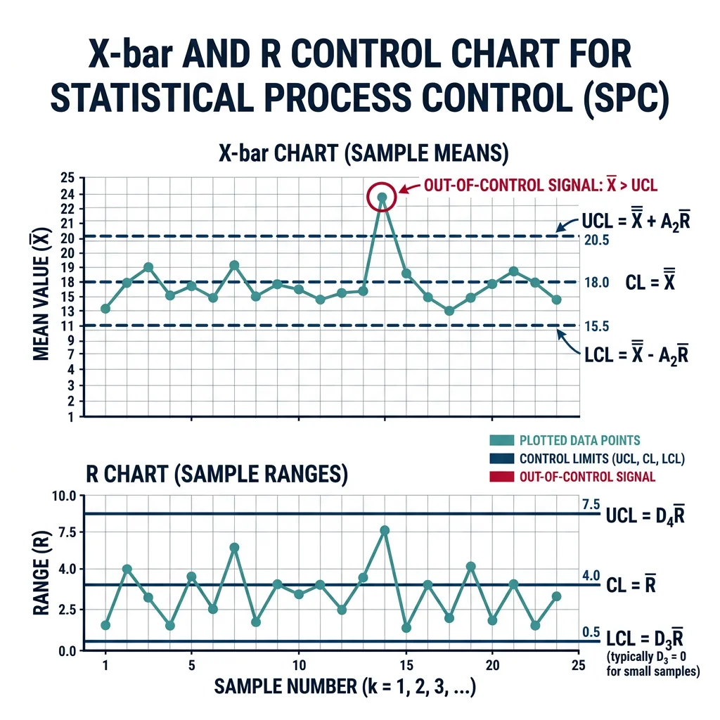
| Control Chart | Data Type | What It Monitors | Control Limits | Example Application |
|---|---|---|---|---|
| X̄ and R Chart | Continuous (subgroups n=2-10) | Process mean and range | UCL = X̿ + A₂R̄, LCL = X̿ - A₂R̄ | Bearing bore diameter (±0.005 mm) |
| X̄ and S Chart | Continuous (subgroups n>10) | Process mean and std deviation | UCL = X̿ + A₃S̄, LCL = X̿ - A₃S̄ | CNC machined shaft diameters |
| p-Chart | Attribute (proportion defective) | Fraction of defective items | UCL = p̄ + 3√(p̄(1-p̄)/n) | PCB solder joint pass/fail rate |
| c-Chart | Attribute (count of defects) | Number of defects per unit | UCL = c̄ + 3√c̄ | Paint defects per car body panel |
| CUSUM Chart | Continuous | Cumulative sum of deviations | V-mask or decision interval | Detecting small persistent shifts |
import numpy as np

# X-bar and R Control Chart Simulator
# Simulates a manufacturing process with a mean shift at sample 15

np.random.seed(42)
n_subgroups = 25     # number of subgroups
subgroup_size = 5    # samples per subgroup
target = 50.000      # mm target dimension
sigma = 0.008        # mm process std dev

# Generate data — normal for first 14, shifted for 15-25
data = np.zeros((n_subgroups, subgroup_size))
for i in range(n_subgroups):
    shift = 0.015 if i >= 14 else 0  # 1.875σ shift at sample 15
    data[i] = np.random.normal(target + shift, sigma, subgroup_size)

# Calculate X-bar and R for each subgroup
x_bars = data.mean(axis=1)
ranges = data.max(axis=1) - data.min(axis=1)

# Overall statistics
x_double_bar = x_bars.mean()
r_bar = ranges.mean()

# Control chart constants for n=5
A2 = 0.577  # X-bar chart
D3 = 0.0    # R chart lower
D4 = 2.114  # R chart upper

# Control limits
UCL_xbar = x_double_bar + A2 * r_bar
LCL_xbar = x_double_bar - A2 * r_bar
UCL_R = D4 * r_bar
LCL_R = D3 * r_bar

print("X-bar and R Control Chart Analysis")
print("=" * 60)
print(f"Grand Mean (X̿):     {x_double_bar:.4f} mm")
print(f"Average Range (R̄):  {r_bar:.5f} mm")
print(f"UCL (X̄):            {UCL_xbar:.4f} mm")
print(f"LCL (X̄):            {LCL_xbar:.4f} mm")
print(f"UCL (R):             {UCL_R:.5f} mm")
print(f"\n{'Subgroup':<10} {'X̄':<12} {'R':<12} {'Status'}")
print("-" * 50)

out_of_control = []
for i in range(n_subgroups):
    status = "OK"
    if x_bars[i] > UCL_xbar or x_bars[i] < LCL_xbar:
        status = "*** OUT OF CONTROL ***"
        out_of_control.append(i + 1)
    print(f"{i+1:<10} {x_bars[i]:<12.4f} {ranges[i]:<12.5f} {status}")

print(f"\nOut-of-control subgroups: {out_of_control}")
print(f"Action: Investigate root cause of mean shift starting at subgroup 15")
Process Capability (Cp/Cpk/Pp/Ppk)
While control charts monitor process stability, capability indices quantify whether a stable process can actually meet the customer's specification limits. A process can be perfectly stable but still produce defects if its natural variation exceeds the tolerance band.
Cp (Potential Capability)
Cp = (USL - LSL) / 6σ
Measures the spread relationship — can the tolerance window contain the process spread? Cp ≥ 1.33 is the typical minimum; automotive (IATF 16949) often requires Cp ≥ 1.67. Cp ignores centering — a biased process can have high Cp but still make defects.
Cpk (Actual Capability)
Cpk = min[(USL - X̄) / 3σ, (X̄ - LSL) / 3σ]
Accounts for centering — penalizes the process if the mean is off-center. Cpk ≤ Cp always. When Cpk = Cp, the process is perfectly centered. When Cpk < 1.0, the process is producing defects.
| Cpk Value | Sigma Level | Defect Rate (PPM) | Industry Standard |
|---|---|---|---|
| 0.67 | 2σ | 45,500 | Unacceptable — immediate action required |
| 1.00 | 3σ | 2,700 | Minimum for non-critical features |
| 1.33 | 4σ | 63 | Standard industry minimum |
| 1.67 | 5σ | 0.57 | Automotive (IATF 16949), aerospace |
| 2.00 | 6σ | 0.002 | Six Sigma target — world class |
Measurement System Analysis (MSA)
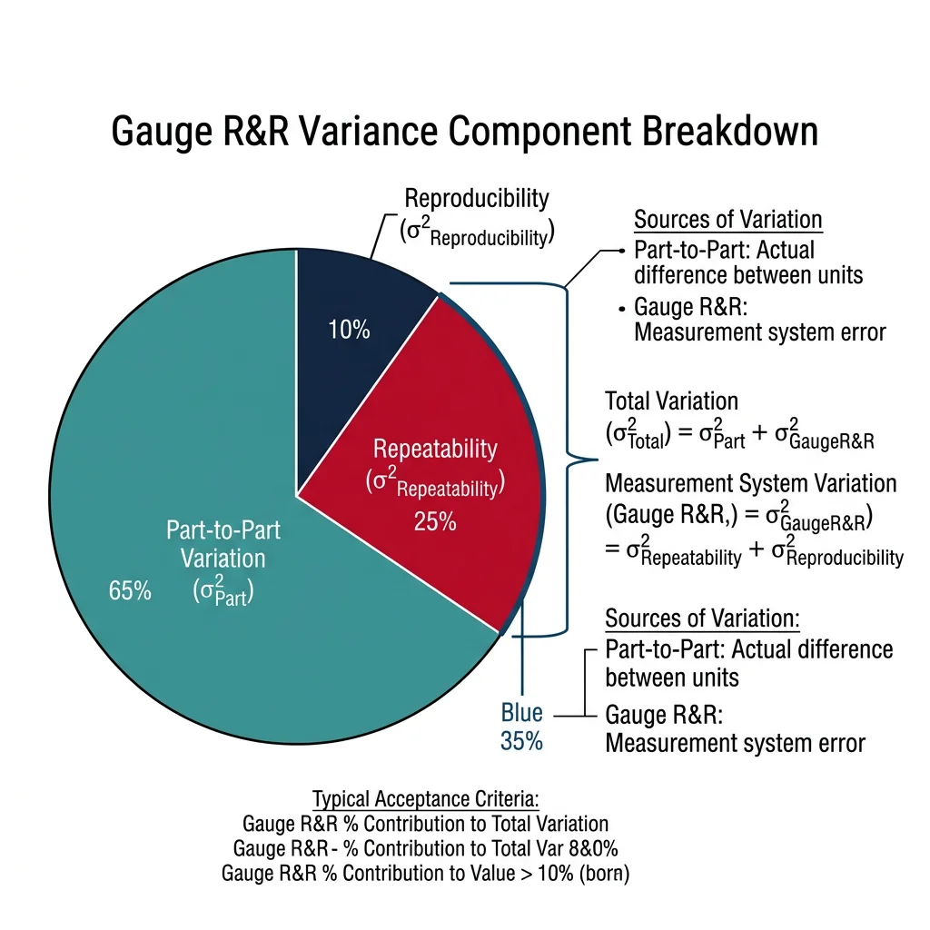
MSA answers a critical question: how much of the observed variation is real process variation vs measurement system noise? If your gauge contributes 30% of total variation, your SPC charts are monitoring the gauge as much as the process. The standard tool is the Gauge R&R (Repeatability & Reproducibility) study.
import numpy as np

# Gauge R&R (Repeatability & Reproducibility) Study
# Crossed design: 3 operators, 10 parts, 3 trials each

np.random.seed(123)
n_operators = 3
n_parts = 10
n_trials = 3
tolerance = 0.050  # mm total tolerance band

# Generate simulated measurement data
part_values = np.random.normal(25.000, 0.008, n_parts)  # true part variation
operator_bias = [0.0, 0.002, -0.001]  # systematic operator differences
gauge_noise = 0.003  # repeatability std dev

measurements = np.zeros((n_operators, n_parts, n_trials))
for op in range(n_operators):
    for part in range(n_parts):
        for trial in range(n_trials):
            measurements[op, part, trial] = (
                part_values[part] + operator_bias[op] +
                np.random.normal(0, gauge_noise)
            )

# Calculate variance components
grand_mean = measurements.mean()

# Repeatability (within operator, within part)
repeatability_var = np.mean([
    measurements[op, part, :].var(ddof=1)
    for op in range(n_operators)
    for part in range(n_parts)
])

# Reproducibility (between operators)
operator_means = measurements.mean(axis=(1, 2))
reproducibility_var = operator_means.var(ddof=1)

# Part variation
part_means = measurements.mean(axis=(0, 2))
part_var = part_means.var(ddof=1)

# Total GRR
grr_var = repeatability_var + reproducibility_var
total_var = grr_var + part_var

# Results
grr_sigma = np.sqrt(grr_var) * 5.15  # 5.15 for 99% confidence
ptv_sigma = np.sqrt(part_var) * 5.15
total_sigma = np.sqrt(total_var) * 5.15

pct_grr_tv = (grr_sigma / total_sigma) * 100
pct_grr_tol = (grr_sigma / tolerance) * 100
ndc = int(1.41 * (ptv_sigma / grr_sigma))  # number of distinct categories

print("Gauge R&R Study Results")
print("=" * 60)
print(f"Repeatability (Equipment Variation):  σ = {np.sqrt(repeatability_var)*1000:.2f} μm")
print(f"Reproducibility (Operator Variation): σ = {np.sqrt(reproducibility_var)*1000:.2f} μm")
print(f"GRR (Total Gauge Variation):          σ = {np.sqrt(grr_var)*1000:.2f} μm")
print(f"Part Variation:                       σ = {np.sqrt(part_var)*1000:.2f} μm")
print(f"\n%GRR (of Total Variation): {pct_grr_tv:.1f}%")
print(f"%GRR (of Tolerance):       {pct_grr_tol:.1f}%")
print(f"Number of Distinct Categories (ndc): {ndc}")
print(f"\nVerdict: {'ACCEPTABLE' if pct_grr_tol < 30 else 'UNACCEPTABLE'}")
print(f"(ndc ≥ 5 required for adequate discrimination, got {ndc})")
Dimensional Metrology
Dimensional metrology is the science of measuring physical dimensions — lengths, angles, positions, and geometric relationships. In manufacturing, every dimension has a tolerance, and metrology determines whether parts are within specification. Modern metrology combines contact probing (tactile) with non-contact scanning (optical, laser) to capture complete part geometry.
| Instrument | Measurement Range | Resolution | Accuracy | Application |
|---|---|---|---|---|
| CMM (touch probe) | 1-3 meters | 0.1 μm | ±1.5 + L/400 μm | Prismatic parts, datum-referenced GD&T |
| CMM (scanning probe) | 1-3 meters | 0.5 μm | ±2.5 μm | Freeform surfaces, profiles, curves |
| Laser tracker | 0-80 meters | 0.1 μm | ±15 + 6L μm | Large assemblies, aircraft, tooling alignment |
| Structured light scanner | 50mm-2m FOV | 5-50 μm | ±10-50 μm | Full-surface digitizing, reverse engineering |
| CT Scanner (industrial) | 10mm-600mm | 1-50 μm | ±5-10 μm | Internal features, AM porosity, assemblies |
| Optical comparator | Profile projection | 5 μm | ±10 μm | 2D profile inspection, thread forms |
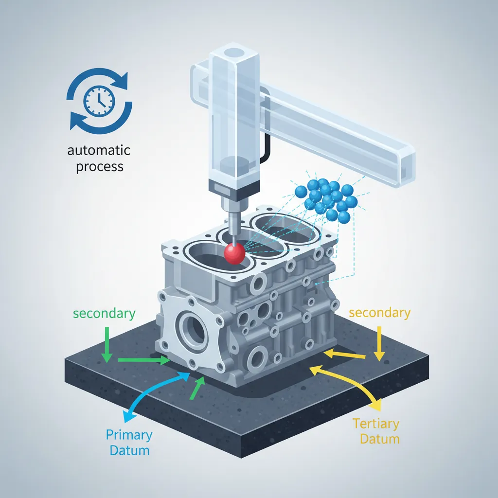
Case Study: CMM in Automotive Engine Block Inspection
A modern engine block has 200+ critical dimensions (bore diameters, deck flatness, bearing housing positions, bolt hole positions). A typical CMM inspection program:
- Setup: Part fixtured on CMM table, aligned using 3-2-1 datum reference frame (3 points on primary datum A, 2 on B, 1 on C)
- Probing strategy: 50-100 points per cylinder bore for roundness, 25+ points per deck face for flatness
- Cycle time: Full program runs 15-45 minutes per block (automated, unattended)
- Output: Pass/fail report with balloon dimensions, statistical data feed to SPC system
- Tolerance example: Cylinder bore diameter 86.000 ±0.010 mm, roundness ≤ 0.005 mm, cylindricity ≤ 0.008 mm
Surface Metrology & Roughness
Surface texture directly affects part function — friction, wear, fatigue life, sealing, appearance, and lubrication retention. Surface roughness is characterized by parameters defined in ISO 4287 and ASME B46.1:
| Parameter | Definition | Typical Values | Application |
|---|---|---|---|
| Ra | Arithmetic average roughness | 0.05-25 μm | Most common parameter, general specification |
| Rz | Average maximum height (5 peaks/valleys) | 0.2-100 μm | Better for surfaces with isolated peaks/scratches |
| Rq (RMS) | Root mean square roughness | 1.1×Ra typically | Statistical applications, optical surfaces |
| Rsk | Skewness (asymmetry of profile) | -1 to +1 | Rsk < 0 → plateaus (good for bearing surfaces) |
| Rku | Kurtosis (sharpness of profile) | ~3.0 (Gaussian) | Rku > 3 → sharp peaks (scratch-sensitive) |
Tolerance Stack-Up & GD&T
Tolerance stack-up analysis predicts whether an assembly will function when individual part tolerances accumulate. In a stack of 10 parts, each with ±0.05 mm tolerance, the worst-case accumulation is ±0.50 mm — but statistical analysis (RSS method) shows the likely accumulation is only ±0.16 mm.
import numpy as np

# Tolerance Stack-Up Analysis
# Worst-Case vs Statistical (RSS) Method
# Example: 5-part linear assembly

dimensions = [
    {"name": "Part A", "nominal": 25.00, "tol": 0.05},
    {"name": "Part B", "nominal": 12.50, "tol": 0.03},
    {"name": "Part C", "nominal": 8.00, "tol": 0.04},
    {"name": "Part D", "nominal": 30.00, "tol": 0.05},
    {"name": "Part E", "nominal": 15.00, "tol": 0.02},
]

assembly_spec = {"nominal": 90.50, "tol": 0.12}  # required assembly tolerance

# Worst-case method: all tolerances add linearly
nominal_sum = sum(d["nominal"] for d in dimensions)
wc_tol = sum(d["tol"] for d in dimensions)

# RSS (Root Sum of Squares) method: statistical combination
rss_tol = np.sqrt(sum(d["tol"]**2 for d in dimensions))

# Monte Carlo simulation: 100,000 random assemblies
n_sim = 100_000
assembly_dims = np.zeros(n_sim)
for d in dimensions:
    # Assume normal distribution, tolerance = 3σ (99.73%)
    sigma = d["tol"] / 3
    assembly_dims += np.random.normal(d["nominal"], sigma, n_sim)

mc_mean = assembly_dims.mean()
mc_std = assembly_dims.std()
mc_tol_3sigma = 3 * mc_std

# Yield calculation
lower_limit = assembly_spec["nominal"] - assembly_spec["tol"]
upper_limit = assembly_spec["nominal"] + assembly_spec["tol"]
in_spec = np.sum((assembly_dims >= lower_limit) & (assembly_dims <= upper_limit))
yield_pct = (in_spec / n_sim) * 100

print("Tolerance Stack-Up Analysis")
print("=" * 60)
print(f"\n{'Part':<10} {'Nominal':<12} {'Tolerance (±)'}")
print("-" * 35)
for d in dimensions:
    print(f"{d['name']:<10} {d['nominal']:<12.2f} ±{d['tol']:.3f} mm")

print(f"\n{'Assembly Nominal:':<30} {nominal_sum:.2f} mm")
print(f"{'Assembly Spec:':<30} {assembly_spec['nominal']:.2f} ±{assembly_spec['tol']:.3f} mm")
print(f"\n{'Method':<25} {'Tolerance (±mm)':<18} {'Within Spec?'}")
print("-" * 55)
print(f"{'Worst-Case:':<25} ±{wc_tol:.3f}           {'YES' if wc_tol <= assembly_spec['tol'] else 'NO — REDESIGN'}")
print(f"{'RSS (Statistical):':<25} ±{rss_tol:.3f}           {'YES' if rss_tol <= assembly_spec['tol'] else 'NO — REDESIGN'}")
print(f"{'Monte Carlo (3σ):':<25} ±{mc_tol_3sigma:.3f}           {'YES' if mc_tol_3sigma <= assembly_spec['tol'] else 'NO — REDESIGN'}")
print(f"\nMonte Carlo Assembly Yield: {yield_pct:.2f}% ({in_spec}/{n_sim} in spec)")
print(f"Monte Carlo Mean: {mc_mean:.4f} mm, Std Dev: {mc_std:.4f} mm")
Non-Destructive Testing
Non-Destructive Testing (NDT) detects internal and surface defects without damaging the part. NDT is mandatory in aerospace, nuclear, pressure vessel, and structural steel industries — where a missed crack can lead to catastrophic failure. NDT technicians are certified under ASNT SNT-TC-1A (USA) or ISO 9712 (international) at Levels I, II, and III.
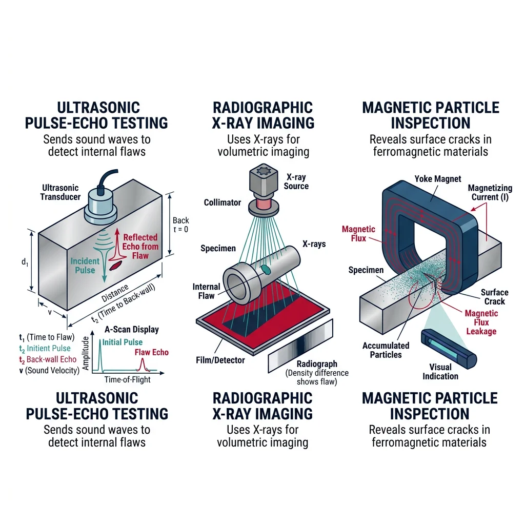
| NDT Method | Defect Type | Materials | Detection Limit | Advantages | Limitations |
|---|---|---|---|---|---|
| Ultrasonic (UT) | Internal voids, cracks, inclusions | Metals, composites, ceramics | 0.5 mm flaw | Deep penetration (>1m), portable, precise depth info | Requires coupling medium, operator skill-dependent |
| Phased Array UT | Same as UT + complex geometries | All UT materials | 0.3 mm flaw | Sector/linear scanning, real-time imaging, weld inspection | Expensive equipment, requires calibration |
| Radiographic (RT) | Porosity, inclusions, incomplete fusion | All (varies by density) | 2% wall thickness | Permanent film record, volumetric detection | Radiation safety, cannot detect tight cracks |
| Computed Tomography | Complete 3D internal structure | All (limited by density/size) | 5-50 μm voxel | 3D defect mapping, dimensional + defect in one scan | Very expensive, limited part size, slow |
Magnetic Particle & Eddy Current
Magnetic Particle Inspection (MPI/MT) detects surface and near-surface cracks in ferromagnetic materials (steel, iron, nickel). The part is magnetized, and iron oxide particles (applied as dry powder or fluorescent wet suspension) accumulate at crack-induced magnetic flux leakage points, making defects visible under UV light.
Eddy Current Testing (ET) induces alternating current in a conductive material via an electromagnetic coil. Defects (cracks, corrosion, material property changes) alter the eddy current flow pattern, which is detected as impedance changes. Eddy current is fast (100+ parts/hour), non-contact, and excellent for detecting surface cracks in non-ferromagnetic materials like aluminum aircraft skins.
Case Study: Aircraft Wing Spar Inspection
Every commercial aircraft wing spar undergoes mandatory NDT at intervals defined by the Structural Inspection Program:
- Fastener hole inspection: Eddy current bolt-hole probes check for fatigue cracks radiating from 2,000+ rivet holes per wing — cracks as small as 0.5 mm must be detected
- Scanning speed: Automated rotating probe inspects each hole in <2 seconds, entire wing in 4-6 hours
- Criticality: Aloha Airlines Flight 243 (1988) — fatigue cracks at rivet holes caused fuselage section to separate in flight. This accident revolutionized structural inspection requirements.
Visual, Dye Penetrant & Acoustic Emission
Visual inspection (VT) is the simplest, cheapest, and most widely used NDT method — every weld, casting, and machined surface gets visual inspection first. Trained inspectors with proper lighting (1,000+ lux) and magnification (up to 10×) can detect surface cracks, porosity, undercut, spatter, and dimensional deviations.
Dye Penetrant Inspection (PT/DPI) detects open-to-surface cracks in any non-porous material (metals, ceramics, plastics):
- Clean the surface thoroughly
- Apply penetrant (red visible or fluorescent) — dwell time 5-30 minutes
- Remove excess penetrant from surface (water-washable or solvent-removable)
- Apply developer (white powder) — draws penetrant out of cracks by capillary action
- Inspect — red indications on white background (or glowing under UV for fluorescent)
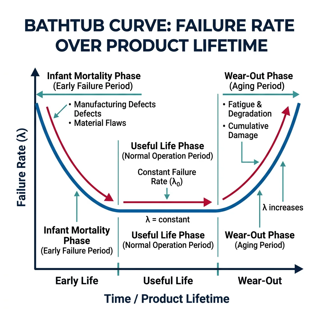
Reliability & Experimental Design
Reliability engineering quantifies the probability that a product or component will perform its intended function without failure for a specified time under stated conditions. Manufacturing quality ensures parts meet specifications at time zero; reliability ensures they continue to meet specifications over their service life.
FMEA: Failure Mode & Effects Analysis
FMEA systematically identifies potential failures and prioritizes them by RPN = Severity × Occurrence × Detection (each 1-10 scale, max RPN = 1,000):
| Component | Failure Mode | Effect | S | O | D | RPN | Action |
|---|---|---|---|---|---|---|---|
| Hydraulic seal | Crack/tear | Fluid leak, loss of pressure | 8 | 4 | 6 | 192 | Add 100% pressure test |
| Bearing | Spalling | Noise, vibration, seizure | 7 | 3 | 5 | 105 | Improve lubrication spec |
| Brake rotor | Fatigue crack | Reduced braking, safety | 10 | 2 | 7 | 140 | UT inspection, shot peen |
| PCB solder | Cold joint | Intermittent connection | 6 | 5 | 4 | 120 | Thermal profiling, AOI |
Priority: Address highest RPN first, but ALWAYS address any failure mode with Severity ≥ 9 regardless of RPN (safety-critical items).
Root Cause Analysis (8D, 5 Whys, Ishikawa)
When defects escape to the customer, Root Cause Analysis (RCA) determines WHY the failure occurred and prevents recurrence. The most widely used structured frameworks:
5 Whys
Ask "Why?" iteratively until the root cause is found (usually 5 levels deep). Example: Bearing failed → Why? Insufficient lubrication → Why? Grease port blocked → Why? Metal chip from machining → Why? Parts not cleaned after machining → Root Cause: Missing wash step in process routing.
flowchart LR
    D1["D1\nTeam"] --> D2["D2\nProblem\nDescription"]
    D2 --> D3["D3\nContainment\nActions"]
    D3 --> D4["D4\nRoot Cause\nAnalysis"]
    D4 --> D5["D5\nCorrective\nActions"]
    D5 --> D6["D6\nVerify\nEffectiveness"]
    D6 --> D7["D7\nPrevent\nRecurrence"]
    D7 --> D8["D8\nCelebrate\nTeam"]
Ishikawa (Fishbone)
Categorize potential causes under 6M branches: Man, Machine, Material, Method, Measurement, Mother Nature (Environment). Team brainstorms causes in each category, then validates with data. Visual diagram makes it easy to communicate during cross-functional investigations.
8D Report
Structured 8-step corrective action process: D1 Team, D2 Problem Description, D3 Containment, D4 Root Cause, D5 Corrective Actions, D6 Verify, D7 Prevent Recurrence, D8 Celebrate. Required by automotive OEMs for supplier quality complaints.
Design of Experiments (DOE)
DOE systematically varies multiple process factors simultaneously to determine which factors significantly affect the output — and their optimal settings. Instead of changing one factor at a time (OFAT), DOE tests combinations to reveal interactions between factors that OFAT completely misses.
import numpy as np

# 2^3 Full Factorial DOE — CNC Milling Surface Roughness
# Factors: Speed (A), Feed (B), Depth of Cut (C)
# Response: Surface Roughness Ra (μm)

factors = {
    "A: Speed (rpm)":     {"low": 1000, "high": 3000},
    "B: Feed (mm/min)":   {"low": 100,  "high": 300},
    "C: Depth (mm)":      {"low": 0.5,  "high": 2.0},
}

# Coded design matrix (-1 = low, +1 = high) for 2^3 factorial
design = np.array([
    [-1, -1, -1],
    [+1, -1, -1],
    [-1, +1, -1],
    [+1, +1, -1],
    [-1, -1, +1],
    [+1, -1, +1],
    [-1, +1, +1],
    [+1, +1, +1],
])

# Measured surface roughness Ra (μm) for each run
# (simulated realistic responses)
Ra = np.array([1.8, 0.9, 3.2, 1.6, 2.4, 1.2, 4.1, 2.8])

n = len(Ra)

# Calculate main effects and interactions
effect_A = np.mean(Ra[design[:, 0] == 1]) - np.mean(Ra[design[:, 0] == -1])
effect_B = np.mean(Ra[design[:, 1] == 1]) - np.mean(Ra[design[:, 1] == -1])
effect_C = np.mean(Ra[design[:, 2] == 1]) - np.mean(Ra[design[:, 2] == -1])

# Interaction effects
AB = design[:, 0] * design[:, 1]
AC = design[:, 0] * design[:, 2]
BC = design[:, 1] * design[:, 2]

effect_AB = np.mean(Ra[AB == 1]) - np.mean(Ra[AB == -1])
effect_AC = np.mean(Ra[AC == 1]) - np.mean(Ra[AC == -1])
effect_BC = np.mean(Ra[BC == 1]) - np.mean(Ra[BC == -1])

print("2^3 Full Factorial DOE — Surface Roughness Optimization")
print("=" * 60)
print(f"\n{'Run':<6} {'Speed':<10} {'Feed':<10} {'Depth':<10} {'Ra (μm)'}")
print("-" * 46)
labels = ["Low", "High"]
for i in range(n):
    s = labels[int((design[i, 0] + 1) / 2)]
    f = labels[int((design[i, 1] + 1) / 2)]
    d = labels[int((design[i, 2] + 1) / 2)]
    print(f"{i+1:<6} {s:<10} {f:<10} {d:<10} {Ra[i]:.1f}")

print(f"\nFactor Effects (change in Ra, μm):")
print(f"  A (Speed):       {effect_A:+.2f}  {'*** SIGNIFICANT' if abs(effect_A) > 0.5 else ''}")
print(f"  B (Feed):        {effect_B:+.2f}  {'*** SIGNIFICANT' if abs(effect_B) > 0.5 else ''}")
print(f"  C (Depth):       {effect_C:+.2f}  {'*** SIGNIFICANT' if abs(effect_C) > 0.5 else ''}")
print(f"  AB interaction:  {effect_AB:+.2f}")
print(f"  AC interaction:  {effect_AC:+.2f}")
print(f"  BC interaction:  {effect_BC:+.2f}")
print(f"\nOptimal Settings for MINIMUM Ra:")
print(f"  Speed:  HIGH (3000 rpm) — effect is {effect_A:+.2f}")
print(f"  Feed:   LOW (100 mm/min) — effect is {effect_B:+.2f}")
print(f"  Depth:  LOW (0.5 mm) — effect is {effect_C:+.2f}")
print(f"  Predicted optimal Ra ≈ {np.mean(Ra) + 0.5*(effect_A - effect_B - effect_C):.1f} μm")