1. Introduction
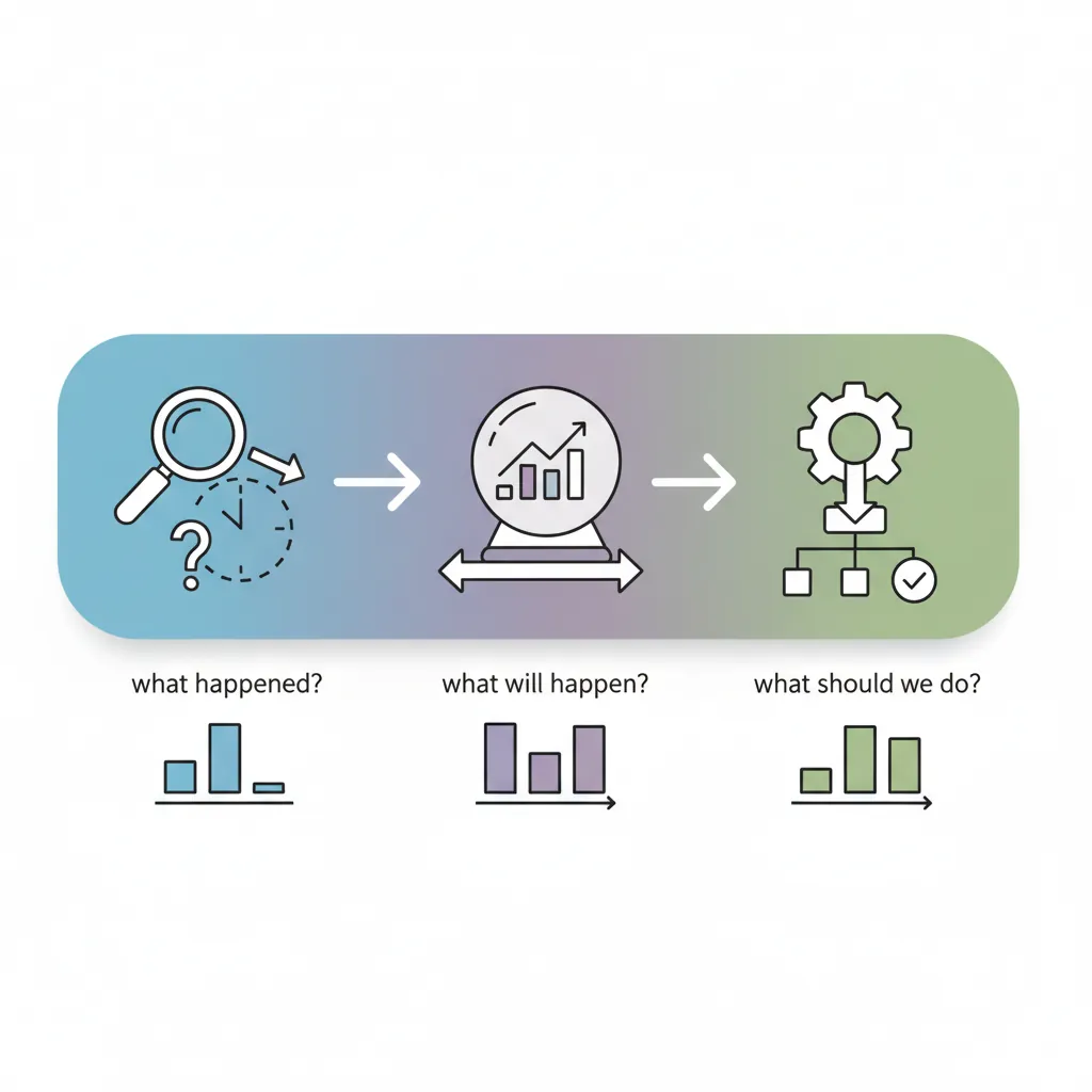
Predictive analytics uses historical data to forecast future outcomes. Unlike descriptive analytics (what happened) or diagnostic analytics (why it happened), predictive analytics answers: What will likely happen next?
Data-Driven Decisions
Introduction to Business Analytics & DDDM
Analytics maturity, data-driven culture, business valueDefining & Tracking KPIs
OKRs, leading/lagging indicators, scorecard designDashboard Design & BI Tools
Tableau, Power BI, dashboard best practices, data vizExperimentation & A/B Testing
Hypothesis testing, control groups, sample sizingStatistical Significance & Interpretation
P-values, confidence intervals, effect size, power analysisDecision Frameworks & Structured Decision Making
Decision matrices, Bayesian thinking, risk analysisData Collection & Quality Management
Surveys, ETL, data governance, cleaning pipelinesBusiness Storytelling & Visualization
Narrative structure, chart selection, audience designPredictive Analytics & Forecasting
Regression, time series, ML models, forecasting methodsData-Driven Culture & Organizational Adoption
Change management, data literacy, organizational buy-inFunction-Specific Data Applications
Marketing, finance, operations, HR analyticsCapstone Projects (Portfolio-Ready)
End-to-end analytics projects, portfolio buildingAdvanced Analytics & Automation
ML pipelines, AutoML, real-time analytics, AI integrationPredictive vs. Descriptive Analytics
| Analytics Type | Question | Example |
|---|---|---|
| Descriptive | What happened? | Last month's sales were $2.3M |
| Diagnostic | Why did it happen? | Sales dropped because of supply issues |
| Predictive | What will happen? | Next quarter revenue will be $7.2M ± $0.5M |
| Prescriptive | What should we do? | Increase inventory by 15% to capture demand |
Business Use Cases
- Revenue forecasting: Project quarterly/annual revenue for planning
- Demand planning: Predict product demand for inventory management
- Churn prediction: Identify customers likely to leave
- Lead scoring: Rank prospects by purchase probability
- Fraud detection: Flag suspicious transactions
- Capacity planning: Predict resource needs
2. Time Series Analysis
A time series is data collected at regular intervals over time. Understanding its components is essential for forecasting.
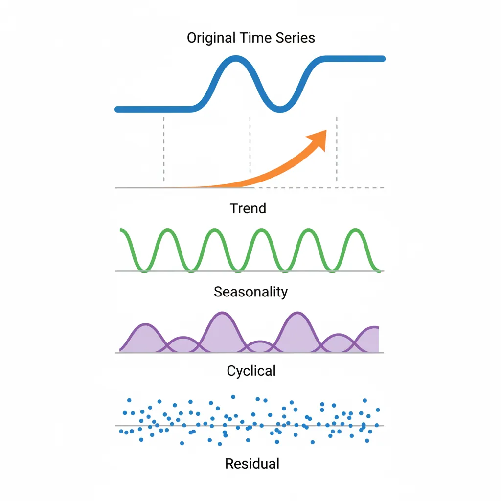
Time Series Components
- Trend: Long-term direction (upward, downward, or flat)
- Seasonality: Regular, predictable patterns (daily, weekly, yearly)
- Cyclical: Irregular, longer-term fluctuations (economic cycles)
- Residual/Noise: Random variation that can't be explained
Time Series Decomposition
OBSERVED DATA = Trend + Seasonality + Residual

    ▲ Sales
    │    ╱╲    ╱╲    ╱╲    ╱╲   ← Observed (jagged)
    │   ╱  ╲  ╱  ╲  ╱  ╲  ╱  ╲
    │  ╱    ╲╱    ╲╱    ╲╱    ╲
    │ ─────────────────────────   ← Trend (smooth)
    │
    └─────────────────────────── Time

Additive model:  Y = T + S + R
Multiplicative:  Y = T × S × R
Decomposition Methods
Common approaches:
- Classical decomposition: Moving average to extract trend, then seasonal
- STL decomposition: Robust method using LOESS smoothing
- X-13ARIMA: Census Bureau method for economic data
Stationarity
A stationary time series has constant statistical properties over time (mean, variance). Many forecasting methods require stationarity.
Making data stationary:
- Differencing: Y'ₜ = Yₜ - Yₜ₋₁
- Log transformation: Stabilize variance
- Seasonal differencing: Y'ₜ = Yₜ - Yₜ₋₁₂ (for monthly data with yearly seasonality)
3. Forecasting Methods
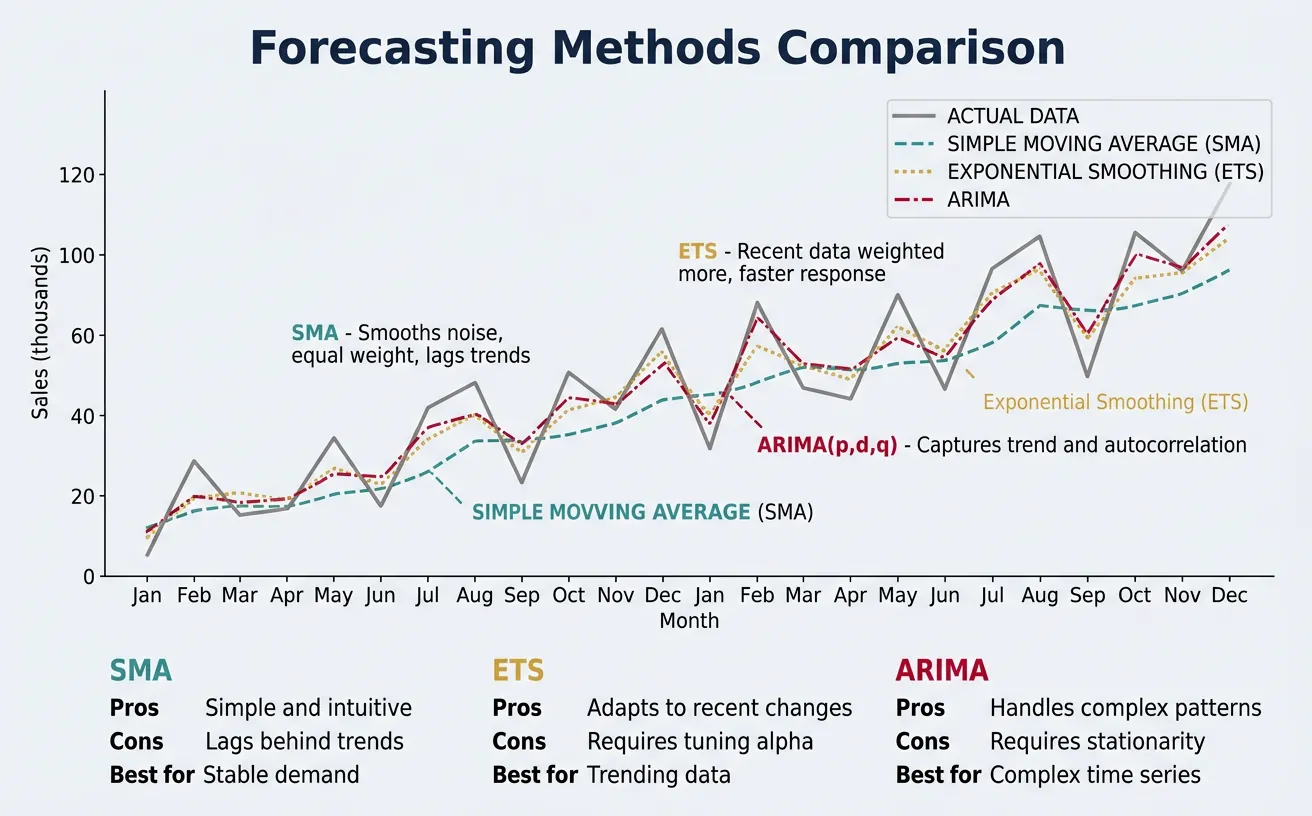
Moving Averages
Simple Moving Average (SMA): Average of the last n periods
graph TD
    START{"Data
Characteristics?"}

    START -->|"Time-series data"| TS{"Seasonality
present?"}
    START -->|"Cross-sectional"| REG["Regression Models
Linear / Logistic"]
    START -->|"Mixed / Complex"| ML["ML Models
XGBoost, Neural Nets"]

    TS -->|"Yes"| SEASON{"Trend
present?"}
    TS -->|"No"| NOSEAS["Simple Moving Average
or Exponential Smoothing"]

    SEASON -->|"Yes"| ARIMA["SARIMA / Holt-Winters
Trend + Seasonal decomposition"]
    SEASON -->|"Seasonal only"| DECOMP["Seasonal Decomposition
STL / X-13"]

    style START fill:#132440,stroke:#132440,color:#fff
    style ARIMA fill:#e8f4f4,stroke:#3B9797
    style ML fill:#f0f4f8,stroke:#16476A
- Pros: Simple, smooths noise
- Cons: Lags behind trends, equal weight to all periods
- Use case: Stable demand with no trend
Exponential Smoothing
Gives more weight to recent observations:
| Method | Components Handled | Use Case |
|---|---|---|
| Simple (SES) | Level only | No trend, no seasonality |
| Holt's | Level + Trend | Trend, no seasonality |
| Holt-Winters | Level + Trend + Seasonality | Trend and seasonality |
ARIMA Models
ARIMA(p, d, q) = AutoRegressive Integrated Moving Average
- p: Autoregressive terms (past values)
- d: Differencing order (to achieve stationarity)
- q: Moving average terms (past errors)
SARIMA adds seasonal components: SARIMA(p,d,q)(P,D,Q)m
4. Regression Models
Linear Regression
Models relationship between dependent variable and one or more predictors:
Y = β₀ + β₁X + ε
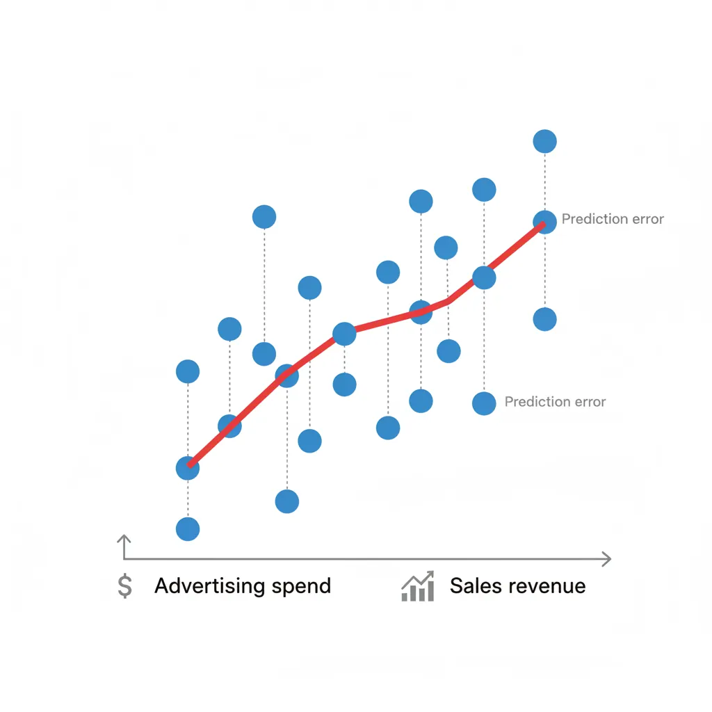
- Use case: Sales vs. advertising spend
- Assumption: Linear relationship, independent errors
Multiple Regression
Multiple predictors: Y = β₀ + β₁X₁ + β₂X₂ + ... + βₙXₙ + ε
- Use case: Revenue predicted by marketing spend, seasonality, economic indicators
- Key metric: Adjusted R² (accounts for number of predictors)
Logistic Regression
For binary outcomes (yes/no, churn/retain):
- Output: Probability between 0 and 1
- Use case: Churn prediction, lead conversion likelihood
5. Machine Learning for Forecasting
Tree-Based Models
- Random Forest: Ensemble of decision trees, handles non-linear relationships
- XGBoost/LightGBM: Gradient boosting, often best performance
- Strengths: Handle complex interactions, feature importance built-in
Neural Networks
- LSTM: Long Short-Term Memory networks for sequential data
- Prophet: Facebook's forecasting library (additive model)
- Use case: Complex patterns, large datasets
When to Use Which Method
- Simple/stable patterns: Moving average, exponential smoothing
- Trend + seasonality: Holt-Winters, SARIMA, Prophet
- Multiple drivers: Regression, tree models
- Complex patterns + large data: Neural networks, XGBoost
6. Accuracy Evaluation
Error Metrics (MAE, RMSE, MAPE)
| Metric | Formula | Interpretation |
|---|---|---|
| MAE | Mean(|Actual - Forecast|) | Average error in same units as data |
| RMSE | √Mean((Actual - Forecast)²) | Penalizes large errors more heavily |
| MAPE | Mean(|Actual - Forecast|/Actual) × 100 | Percentage error (scale-independent) |
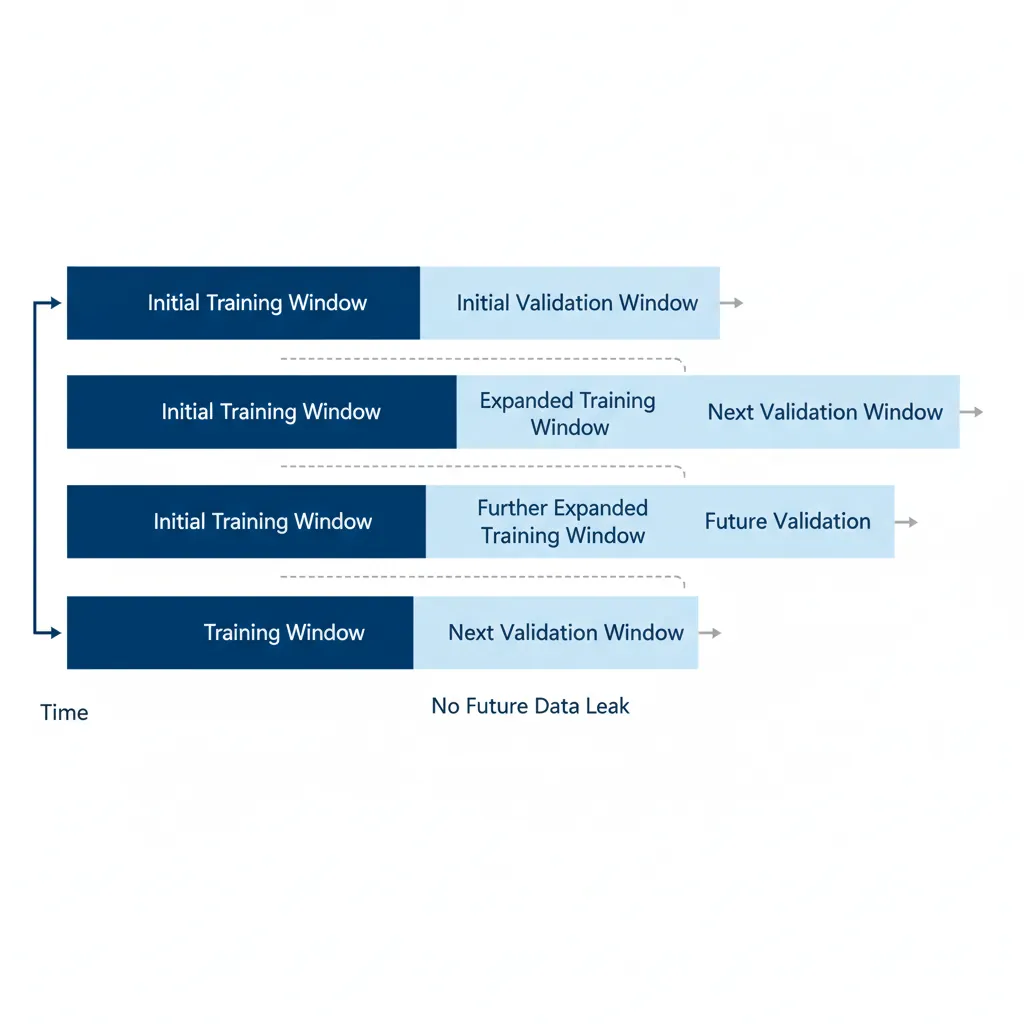
Time Series Cross-Validation
Walk-forward validation: Train on data up to time t, predict t+1, then expand training window and repeat. Never use future data to predict the past!
7. Conclusion & Next Steps
You've now covered the key concepts in this section of data-driven decision making. Here's a summary of what you've learned:
Key Takeaways
- Understand your data: Decompose into trend, seasonality, and residual
- Match method to pattern: Simple patterns → simple methods; complex → ML
- Evaluate properly: Use time-aware cross-validation, not random splits
- Quantify uncertainty: Always provide prediction intervals, not just point forecasts
- Iterate: Forecasting is iterative—review accuracy and refine
In the next article, we'll cover Data-Driven Culture & Organizational Adoption—how to build an organization where data drives decisions at every level.