Stress-Strain & Elastic Behavior
Materials Science Mastery
Atomic Structure & Quantum Foundations
Quantum mechanics, bonding, band theory, Fermi energy, phononsCrystal Structures, Defects & Diffusion
FCC/BCC/HCP, Miller indices, dislocations, phase diagrams, Fick's lawsMetals & Alloys
Iron-carbon diagram, steels, aluminum, titanium, superalloys, heat treatmentPolymers & Soft Materials
Polymer chemistry, thermoplastics, viscoelasticity, rheology, biopolymersCeramics, Glass & Composites
Oxide ceramics, toughening, fiber-reinforced composites, interfacial bondingMechanical Behavior & Testing
Stress-strain, hardness, fatigue, fracture toughness, nanoindentationFailure Analysis & Reliability Engineering
Fractography, corrosion, tribology, root cause analysisNanomaterials & Smart Materials
Nanotubes, graphene, piezoelectrics, shape memory alloys, self-healingMaterials Characterization Techniques
XRD, SEM, TEM, AFM, DSC, TGA, spectroscopyThermodynamics & Kinetics of Materials
Gibbs free energy, CALPHAD, phase stability, solidificationElectronic, Magnetic & Optical Materials
Semiconductors, photovoltaics, dielectrics, superconductorsBiomaterials
Implants, biocompatibility, tissue engineering, drug deliveryEnergy Materials
Battery materials, hydrogen storage, fuel cells, nuclear materialsComputational Materials Science
DFT, molecular dynamics, FEM, materials informatics, AIImagine stretching a rubber band between your fingers. At first, it stretches easily and snaps back when released — that's elastic deformation. Keep pulling harder and it begins to permanently deform — that's plastic deformation. Pull even harder and it snaps — that's fracture. Every material in the world follows this same fundamental story, but the numbers are wildly different. A rubber band stretches 500% before breaking; a ceramic shatters at 0.1% strain. Understanding these differences is what mechanical testing is all about.
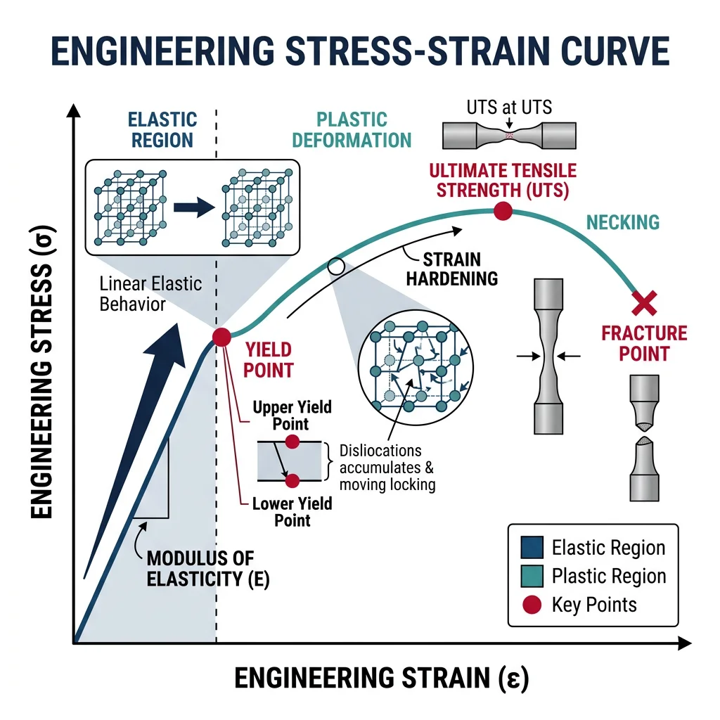
The tensile test is the most fundamental mechanical test in materials science. A standardized specimen (typically a "dog-bone" shape) is gripped at both ends and pulled apart at a controlled rate while instruments measure the applied force and the specimen's elongation. The result is a stress-strain curve — the fingerprint of a material's mechanical behavior.
A typical stress-strain curve for a ductile metal has five distinct regions:
- Linear Elastic Region: Stress is proportional to strain (Hooke's Law). Remove the load and the material returns to its original shape — like an ideal spring.
- Yield Point: The stress at which permanent deformation begins. Some materials (like low-carbon steel) show a distinct upper and lower yield point; others (like aluminum) transition gradually.
- Strain Hardening: After yielding, the material requires increasing stress to continue deforming. Dislocations multiply and tangle, making further deformation harder — like trying to push through an ever-thickening crowd.
- Necking: At the ultimate tensile strength (UTS), deformation localizes in one region and the specimen begins to thin dramatically.
- Fracture: The specimen breaks. Ductile materials form a "cup-and-cone" fracture surface; brittle materials break with a flat, granular surface.
- Young's Modulus (E): Slope of the linear elastic region — a measure of stiffness
- Yield Strength ($\sigma_y$): Stress at onset of permanent deformation
- Ultimate Tensile Strength (UTS / $\sigma_{UTS}$): Maximum engineering stress
- Elongation at Break (% EL): $\frac{L_f - L_0}{L_0} \times 100$ — a measure of ductility
- Reduction in Area (% RA): $\frac{A_0 - A_f}{A_0} \times 100$ — another ductility measure
- Toughness: Total area under the stress-strain curve — energy absorbed before fracture
- Resilience: Area under the elastic portion — energy that can be recovered
import numpy as np
import matplotlib.pyplot as plt

# Simulate a stress-strain curve for mild steel
# Elastic region: sigma = E * epsilon
E = 200e3  # Young's modulus in MPa (200 GPa for steel)
sigma_y = 250  # Yield strength in MPa
sigma_uts = 400  # Ultimate tensile strength in MPa
epsilon_fracture = 0.25  # 25% elongation at break

# Build piecewise stress-strain curve
# Region 1: Linear elastic (0 to yield)
epsilon_y = sigma_y / E
eps_elastic = np.linspace(0, epsilon_y, 100)
sig_elastic = E * eps_elastic

# Region 2: Strain hardening (yield to UTS) using Hollomon equation: sigma = K * eps^n
n = 0.2  # Strain hardening exponent (typical for mild steel)
K = sigma_uts / (0.15 ** n)  # Fit K so UTS occurs near eps=0.15
eps_plastic = np.linspace(epsilon_y, 0.15, 200)
sig_plastic = K * eps_plastic ** n
sig_plastic = np.maximum(sig_plastic, sigma_y)  # Ensure above yield

# Region 3: Necking (UTS to fracture — engineering stress drops)
eps_neck = np.linspace(0.15, epsilon_fracture, 100)
sig_neck = sigma_uts * (1 - 2.5 * (eps_neck - 0.15) ** 1.5)
sig_neck = np.maximum(sig_neck, 100)  # Don't go below fracture stress

# Combine all regions
epsilon = np.concatenate([eps_elastic, eps_plastic, eps_neck])
sigma = np.concatenate([sig_elastic, sig_plastic, sig_neck])

# Plot
plt.figure(figsize=(10, 6))
plt.plot(epsilon * 100, sigma, 'b-', linewidth=2, label='Engineering Stress-Strain')
plt.axhline(y=sigma_y, color='r', linestyle='--', alpha=0.5, label=f'Yield Strength = {sigma_y} MPa')
plt.axhline(y=sigma_uts, color='g', linestyle='--', alpha=0.5, label=f'UTS = {sigma_uts} MPa')
plt.fill_between(eps_elastic * 100, sig_elastic, alpha=0.2, color='cyan', label='Elastic Region (Resilience)')
plt.xlabel('Engineering Strain (%)', fontsize=12)
plt.ylabel('Engineering Stress (MPa)', fontsize=12)
plt.title('Stress-Strain Curve — Mild Steel', fontsize=14)
plt.legend(fontsize=10)
plt.grid(True, alpha=0.3)
plt.annotate('Necking begins', xy=(15, sigma_uts), xytext=(18, sigma_uts + 50),
            arrowprops=dict(arrowstyle='->', color='black'), fontsize=10)
plt.tight_layout()
plt.show()

# Calculate key properties
resilience = 0.5 * sigma_y * epsilon_y  # Area of elastic triangle
toughness = np.trapz(sigma, epsilon)  # Total area under curve
print(f"Young's Modulus: {E/1e3:.0f} GPa")
print(f"Yield Strength: {sigma_y} MPa")
print(f"Ultimate Tensile Strength: {sigma_uts} MPa")
print(f"Elongation at Break: {epsilon_fracture*100:.1f}%")
print(f"Resilience: {resilience:.2f} MJ/m³")
print(f"Toughness: {toughness:.2f} MJ/m³")
Elastic Modulus & Poisson's Ratio
In the elastic region, materials obey Hooke's Law: stress is directly proportional to strain. Think of it like a spring — pull twice as hard, and it stretches twice as far. The proportionality constant is the elastic modulus, one of the most important material properties in engineering.
There are actually three elastic moduli, corresponding to three types of loading:
- Young's Modulus (E): Resistance to uniaxial tension/compression — $\sigma = E\varepsilon$. Think: stretching or squeezing a rod along its length.
- Shear Modulus (G): Resistance to shape distortion — $\tau = G\gamma$. Think: sliding the top of a deck of cards sideways.
- Bulk Modulus (K): Resistance to uniform compression — $P = -K\frac{\Delta V}{V}$. Think: squeezing a ball from all directions underwater.
These are related by: $E = 2G(1 + \nu) = 3K(1 - 2\nu)$, where $\nu$ is Poisson's ratio.
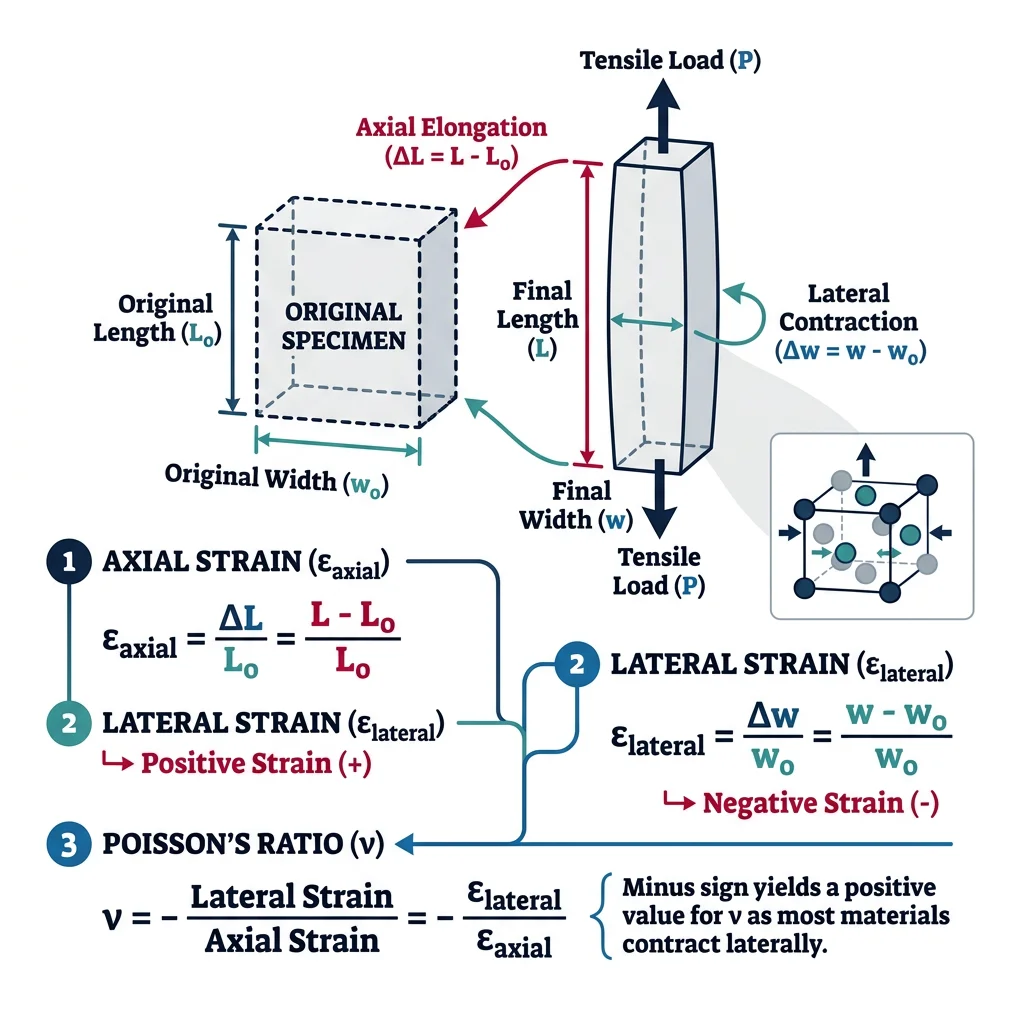
Poisson's ratio ($\nu$) describes how much a material contracts laterally when stretched axially. Imagine pulling a rubber eraser lengthwise — it gets thinner in the other two directions. Mathematically: $\nu = -\frac{\varepsilon_{lateral}}{\varepsilon_{axial}}$. For most engineering materials, $\nu$ ranges from 0.25 to 0.35. Rubber is nearly incompressible at $\nu \approx 0.5$, while cork has $\nu \approx 0$ (which is why it works as a bottle stopper — it doesn't expand sideways when pushed in).
| Material | E (GPa) | G (GPa) | $\nu$ | Typical Use |
|---|---|---|---|---|
| Diamond | 1,050 | 478 | 0.10 | Cutting tools, optics |
| Tungsten Carbide | 620 | 262 | 0.18 | Drill bits, mining tools |
| Steel (mild) | 200 | 80 | 0.30 | Structural beams, bolts |
| Titanium (Ti-6Al-4V) | 114 | 44 | 0.34 | Aerospace, biomedical |
| Aluminum (6061) | 69 | 26 | 0.33 | Aircraft skin, frames |
| Copper | 117 | 45 | 0.34 | Electrical wiring |
| Bone (cortical) | 7–30 | 3 | 0.30 | Skeletal structure |
| HDPE Polymer | 0.8 | – | 0.46 | Bottles, pipes |
| Natural Rubber | 0.001–0.1 | – | 0.50 | Tires, seals |
Yield Strength & Plastic Deformation
The yield strength marks the boundary between recoverable (elastic) and permanent (plastic) deformation. Below the yield stress, atoms return to their equilibrium positions when the load is removed. Above it, atoms permanently rearrange — primarily through dislocation motion.
For most engineering alloys (aluminum, titanium, stainless steel), the transition from elastic to plastic isn't sharp — there's no distinct "pop" at yielding. Instead, engineers use the 0.2% offset method: draw a line parallel to the elastic slope starting at 0.2% strain (0.002). Where this line intersects the stress-strain curve defines the yield strength. This convention provides a consistent, reproducible measurement even when the actual yield transition is gradual.
Case Study: Selecting Metals for Aircraft Wing Skin
An aircraft wing skin must have high yield strength (to resist flight loads without permanent deformation), high fatigue resistance (millions of pressurization cycles), low density (fuel efficiency), and good fracture toughness (damage tolerance). Consider three candidates:
| Property | Al 2024-T3 | Al 7075-T6 | Ti-6Al-4V |
|---|---|---|---|
| Yield Strength (MPa) | 345 | 503 | 880 |
| UTS (MPa) | 483 | 572 | 950 |
| Density (g/cm³) | 2.78 | 2.81 | 4.43 |
| Specific Strength (kN·m/kg) | 124 | 179 | 199 |
| Fracture Toughness (MPa√m) | 37 | 25 | 75 |
| Fatigue Life (relative) | Excellent | Good | Excellent |
Result: Al 2024-T3 dominates for commercial aircraft fuselage skins (excellent fatigue + good toughness). Al 7075-T6 is preferred for upper wing skins (higher strength, compression-dominated loading). Ti-6Al-4V is used for high-load structural attachments where its superior fracture toughness and corrosion resistance justify the higher cost and density.
Hardness & Impact Testing
If you've ever compared scratching glass with a steel nail versus a copper penny, you already understand hardness intuitively — it's a material's resistance to localized plastic deformation (denting, scratching, or indentation). Hardness tests are the fastest, cheapest, and most widely used mechanical tests in industry because they're non-destructive (or nearly so), require minimal specimen preparation, and correlate with other properties like tensile strength.
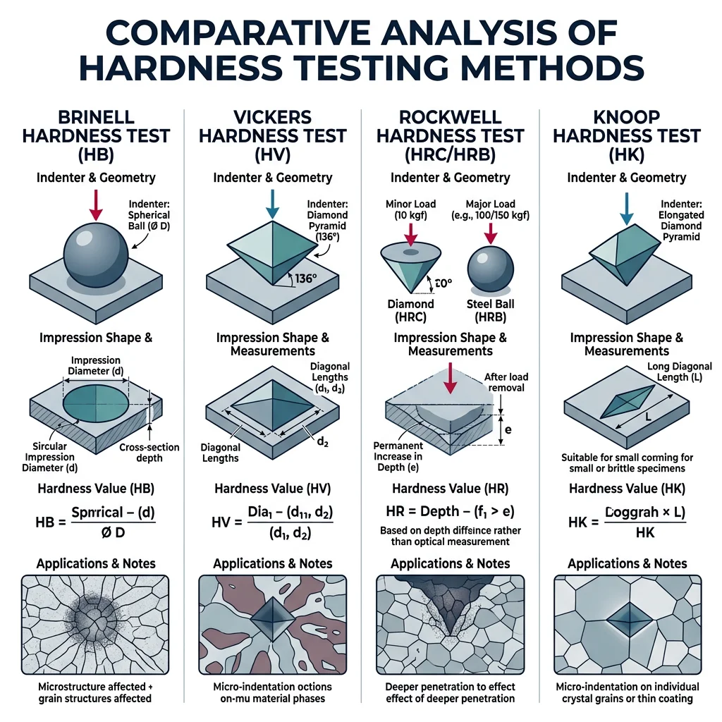
All modern indentation hardness tests work on the same principle: press a hard indenter into the surface under a known load, then measure the size (or depth) of the resulting impression. The differences lie in the indenter geometry and the measurement method:
| Test | Indenter | Load Range | Measurement | Best For | Scale Example |
|---|---|---|---|---|---|
| Brinell (HB) | 10 mm steel or WC ball | 500–3000 kgf | Diameter of imprint | Castings, forgings, rough surfaces | HB 200 (mild steel) |
| Vickers (HV) | Diamond pyramid (136°) | 1 gf – 120 kgf | Diagonal of imprint | Universal — any material, thin sections | HV 800 (hardened tool steel) |
| Rockwell (HR) | Diamond cone or steel ball | 60–150 kgf | Depth of indentation | Quick QC in production, hardened steels (HRC), soft metals (HRB) | HRC 60 (file-hard steel) |
| Knoop (HK) | Elongated diamond pyramid | 1–1000 gf | Long diagonal | Thin coatings, ceramics, brittle materials | HK 2500 (diamond) |
import numpy as np

# Hardness conversion calculator
# Approximate empirical conversions for steels (ASTM E140)
def hrc_to_hv(hrc):
    """Convert Rockwell C to Vickers (valid for HRC 20-65)"""
    return 1.549e-3 * hrc**3 - 0.09212 * hrc**2 + 11.44 * hrc + 202.4

def hv_to_hb(hv):
    """Convert Vickers to Brinell (valid for HV 100-630)"""
    if hv <= 400:
        return 0.9351 * hv + 4.28
    else:
        return 0.832 * hv + 44.0

def hb_to_uts(hb):
    """Estimate UTS (MPa) from Brinell hardness for steels"""
    return 3.45 * hb

# Example conversions
print("=== Hardness Conversion Table (Steels) ===")
print(f"{'HRC':>6} {'HV':>8} {'HB':>8} {'UTS (MPa)':>12}")
print("-" * 38)
for hrc in [20, 25, 30, 35, 40, 45, 50, 55, 60]:
    hv = hrc_to_hv(hrc)
    hb = hv_to_hb(hv)
    uts = hb_to_uts(hb)
    print(f"{hrc:>6} {hv:>8.0f} {hb:>8.0f} {uts:>12.0f}")

print("\n--- Example: Quenched & Tempered 4140 Steel ---")
measured_hrc = 42
hv_val = hrc_to_hv(measured_hrc)
hb_val = hv_to_hb(hv_val)
print(f"Measured: HRC {measured_hrc}")
print(f"≈ HV {hv_val:.0f}")
print(f"≈ HB {hb_val:.0f}")
print(f"≈ UTS {hb_to_uts(hb_val):.0f} MPa ({hb_to_uts(hb_val)/6.895:.0f} ksi)")
Impact Testing & Toughness
Hardness and tensile strength tell you how strong a material is, but they don't tell you how it behaves under sudden, violent loading. A glass window has impressive compressive strength but shatters when struck by a pebble. Impact testing measures a material's resistance to fracture under high-speed loading — its toughness under dynamic conditions.
The two standard impact tests use a pendulum that swings down and strikes a notched specimen:
- Charpy Test: Specimen supported as a horizontal beam; struck behind the notch. The most widely used impact test worldwide (ISO 148, ASTM E23). The specimen is 10 × 10 × 55 mm with a V-notch or U-notch.
- Izod Test: Specimen clamped vertically like a cantilever; struck at the free end above the notch. Common in plastics testing (ASTM D256).
The pendulum's height after breaking the specimen tells you how much energy was absorbed: $E_{absorbed} = mg(h_{initial} - h_{final})$. Tough materials absorb lots of energy (bendable steel: ~100 J); brittle materials absorb very little (cold glass: ~2 J).
Case Study: The Titanic — Cold-Brittle Steel
When the RMS Titanic struck an iceberg on April 14, 1912, the water temperature was approximately −2 °C. Metallurgical analysis of recovered hull plates revealed the steel had a DBTT of about 25–35 °C — well above the water temperature. The steel contained high sulfur content (~0.065 wt%) forming manganese sulfide (MnS) inclusions that acted as crack initiation sites.
Charpy impact tests on recovered samples showed the steel absorbed only ~1 J at 0 °C, compared to ~100 J for modern ship steel at the same temperature. The rivets were even worse — wrought iron with slag stringers that shattered on impact. Rather than bending and absorbing the iceberg's energy, the hull plates fractured in a brittle manner, opening seams between the plates and allowing seawater to flood six compartments.
Modern standards (ABS, Lloyds): Require ship steels to have Charpy values ≥ 27 J at the minimum design temperature, and mandate controlled chemistry (S < 0.005%, high Mn/S ratio) with normalized or TMCP processing.
Nanoindentation Techniques
What if you need to measure the hardness of a thin coating only 500 nm thick, or map the mechanical properties across individual grains in a microstructure? Traditional tests leave indents millimeters wide — far too large. Nanoindentation solves this by pressing a sharp diamond tip (typically a Berkovich indenter — a three-sided pyramid) into the surface with forces as small as micro-Newtons and displacement resolution of sub-nanometers.
The key innovation is the Oliver-Pharr method (1992), which extracts both hardness and elastic modulus from the unloading curve without even needing to image the indent. As the indenter is withdrawn, the initial slope of the unloading curve gives the contact stiffness $S = \frac{dP}{dh}$, which relates to the reduced modulus:
$$E_r = \frac{\sqrt{\pi}}{2\beta} \cdot \frac{S}{\sqrt{A_c}}$$where $A_c$ is the projected contact area (calibrated from the contact depth), $\beta$ is a geometric correction factor (1.034 for Berkovich), and $E_r$ relates to the sample modulus by: $\frac{1}{E_r} = \frac{1 - \nu_s^2}{E_s} + \frac{1 - \nu_i^2}{E_i}$ (accounting for deformation of both sample and diamond indenter).
Fatigue & Fracture
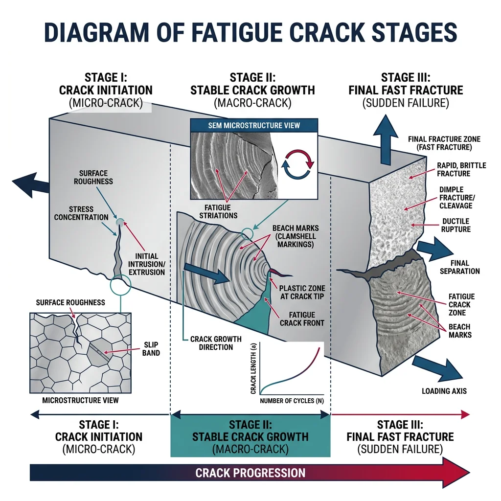
Take a paperclip and bend it back and forth. After fewer than 20 cycles, it snaps — even though you never pulled it anywhere close to its tensile strength. This is fatigue failure: fracture under repeated cyclic loading at stresses well below the yield strength. Fatigue causes an estimated 90% of all mechanical failures in service. It's insidious because it gives little visible warning — a tiny crack nucleates at a stress concentration, grows invisibly for thousands or millions of cycles, and then catastrophically propagates when the remaining cross-section can no longer support the load.
The foundational tool for fatigue design is the S-N curve (stress vs. number of cycles to failure, also called a Wöhler curve). Specimens are subjected to reversed cyclic loading at different stress amplitudes, and the number of cycles to fracture is recorded. The resulting plot typically shows:
- Low-cycle fatigue (LCF): High stress amplitudes, $N_f < 10^4$ cycles. Significant plastic strain each cycle. Common in earthquake loading, engine start-stop cycles.
- High-cycle fatigue (HCF): Lower stresses, $N_f > 10^4$ cycles. Predominantly elastic deformation. The regime most structural components operate in.
- Endurance limit (ferrous metals): Below a critical stress ($S_e$), steel and titanium alloys can theoretically survive infinite cycles. This is a true design threshold — stay below it and fatigue isn't a concern. Typically $S_e \approx 0.4 \text{–} 0.5 \times \sigma_{UTS}$ for steels.
- No endurance limit (non-ferrous): Aluminum, copper, and most polymers have no true endurance limit — they will eventually fail at any cyclic stress given enough cycles. Designers specify fatigue strength at a reference life (e.g., $10^7$ or $10^8$ cycles).
import numpy as np
import matplotlib.pyplot as plt

# Generate and plot S-N curves for steel vs aluminum
N = np.logspace(2, 8, 500)  # Number of cycles (100 to 100 million)

# Steel (4340, quenched & tempered): has endurance limit
sigma_uts_steel = 1000  # MPa
Se_steel = 450  # Endurance limit ~0.45 * UTS
# Basquin equation: S = a * N^b (for N > ~1000)
a_steel = 1800
b_steel = -0.08
S_steel = a_steel * N ** b_steel
S_steel = np.maximum(S_steel, Se_steel)  # Floor at endurance limit

# Aluminum (7075-T6): NO endurance limit
a_alum = 1200
b_alum = -0.10
S_alum = a_alum * N ** b_alum

fig, (ax1, ax2) = plt.subplots(1, 2, figsize=(14, 5))

# S-N Curve
ax1.semilogx(N, S_steel, 'b-', linewidth=2, label='4340 Steel')
ax1.semilogx(N, S_alum, 'r-', linewidth=2, label='7075-T6 Aluminum')
ax1.axhline(y=Se_steel, color='blue', linestyle=':', alpha=0.5, label=f'Steel Endurance Limit = {Se_steel} MPa')
ax1.set_xlabel('Cycles to Failure (N)', fontsize=12)
ax1.set_ylabel('Stress Amplitude (MPa)', fontsize=12)
ax1.set_title('S-N Curves: Steel vs Aluminum', fontsize=13)
ax1.legend(fontsize=9)
ax1.grid(True, alpha=0.3)
ax1.set_ylim(0, 1200)

# Goodman Diagram for the steel
sigma_a_axis = np.linspace(0, Se_steel, 100)
sigma_m_goodman = sigma_uts_steel * (1 - sigma_a_axis / Se_steel)

ax2.plot(sigma_m_goodman, sigma_a_axis, 'b-', linewidth=2, label='Goodman Line')
ax2.fill_between(sigma_m_goodman, sigma_a_axis, alpha=0.15, color='green', label='Safe Region')
ax2.set_xlabel('Mean Stress σ_m (MPa)', fontsize=12)
ax2.set_ylabel('Stress Amplitude σ_a (MPa)', fontsize=12)
ax2.set_title('Goodman Diagram — 4340 Steel', fontsize=13)
ax2.set_xlim(0, sigma_uts_steel * 1.05)
ax2.set_ylim(0, Se_steel * 1.1)
ax2.legend(fontsize=10)
ax2.grid(True, alpha=0.3)

plt.tight_layout()
plt.show()

# Fatigue life prediction
design_stress = 500  # MPa alternating stress
if design_stress > Se_steel:
    N_life = (design_stress / a_steel) ** (1 / b_steel)
    print(f"Predicted fatigue life at {design_stress} MPa: {N_life:.0f} cycles")
else:
    print(f"At {design_stress} MPa: Infinite life (below endurance limit of {Se_steel} MPa)")
Fracture Toughness & LEFM
Fracture mechanics answers a question that tensile testing cannot: "If my component has a crack, how large can that crack be before catastrophic failure?" This is profoundly practical — every real structure contains flaws (inclusions, porosity, machining marks, fatigue cracks). The field was pioneered by A.A. Griffith (1920) for brittle materials and extended by G.R. Irwin (1957) for metals.
In Linear Elastic Fracture Mechanics (LEFM), the stress field near a crack tip is characterized by the stress intensity factor $K$:
$$K_I = Y \sigma \sqrt{\pi a}$$where $\sigma$ is the applied stress, $a$ is the crack half-length, and $Y$ is a dimensionless geometry factor (1.0 for a central crack in an infinite plate, 1.12 for an edge crack). The subscript $I$ denotes Mode I (opening mode — the most common in practice). Fracture occurs when $K_I$ reaches the material's fracture toughness $K_{IC}$ — a true material property measured under plane strain conditions (ASTM E399).
Case Study: The de Havilland Comet — Birth of Fracture Mechanics
In 1954, two de Havilland Comet jet airliners — the world's first commercial jetliner — disintegrated in flight. Investigation revealed fatigue cracks originating from the square corners of the rectangular cabin windows. The sharp corners created extreme stress concentrations (stress intensity factors 3–4× the nominal stress). After ~3,000 pressurization cycles, cracks grew to critical length and the fuselage explosively decompressed.
This catastrophe transformed aircraft design: all modern aircraft use oval or rounded windows (reducing $K$ by ~60%), employ crack-arrest straps (longitudinal doublers that stop running cracks), and follow damage-tolerant design philosophy — assuming cracks exist and ensuring they won't grow to critical size between inspections.
Case Study: Aloha Airlines Flight 243 — Multi-Site Damage
On April 28, 1988, a Boeing 737-200 lost an 18-foot section of its upper fuselage at 24,000 feet. The aircraft had accumulated 89,680 flight cycles — the second-highest cycle count of any 737 in the world. Investigation revealed multi-site fatigue damage (MSD): hundreds of small fatigue cracks at rivet holes along lap joints, individually below detectable limits, but collectively linking up to produce a catastrophic fracture path.
The cold-bonded lap joints had debonded due to corrosion in Hawaii's salty, humid environment, concentrating all load transfer through the rivets. This case established the concepts of widespread fatigue damage (WFD) in aging aircraft structures and led to mandatory corrosion prevention programs and supplemental structural inspections for high-cycle aircraft worldwide.
Crack Growth & Paris Law
Between the initial formation of a fatigue crack and final catastrophic failure lies a period of stable crack growth. The Paris Law (1963) describes the rate of fatigue crack growth per cycle as a function of the stress intensity factor range:
$$\frac{da}{dN} = C(\Delta K)^m$$where $\Delta K = K_{max} - K_{min} = Y\Delta\sigma\sqrt{\pi a}$, and $C$ and $m$ are material constants. For most metals, $m$ ranges from 2 to 4. This law operates in the "Paris regime" (Region II of the da/dN vs. ΔK curve). Below a threshold $\Delta K_{th}$, cracks don't grow; above $K_{IC}$, fracture is instantaneous.
The Paris Law is the backbone of damage-tolerant design: if you know the initial flaw size (from inspection limits), the Paris constants (from testing), and the loading spectrum, you can predict how many cycles it takes for the crack to grow from detectable size to critical size — and schedule inspections accordingly.
import numpy as np
import matplotlib.pyplot as plt

# Paris Law crack growth simulation
# Material: 7075-T6 Aluminum alloy
C = 1.5e-11     # Paris constant (m/cycle, for da/dN in m/cycle, DeltaK in MPa*sqrt(m))
m_paris = 3.1   # Paris exponent
K_IC = 27       # Fracture toughness (MPa*sqrt(m))
delta_K_th = 2  # Threshold stress intensity factor range (MPa*sqrt(m))
Y = 1.12        # Geometry factor (edge crack)

# Loading
delta_sigma = 100  # Stress range (MPa)
initial_crack = 0.5e-3  # Initial crack size: 0.5 mm

# Numerical integration of Paris Law
a = initial_crack
crack_sizes = [a]
cycles = [0]
N = 0
dN = 100  # Cycle increment

while True:
    delta_K = Y * delta_sigma * np.sqrt(np.pi * a)
    K_max = Y * delta_sigma * np.sqrt(np.pi * a)  # R=0 loading

    if K_max >= K_IC:
        print(f"Critical fracture at a = {a*1000:.2f} mm after N = {N:,} cycles")
        break

    if delta_K < delta_K_th:
        dN = 1000
        N += dN
        cycles.append(N)
        crack_sizes.append(a)
        if N > 1e8:
            print("Threshold not exceeded — infinite life")
            break
        continue

    da = C * delta_K ** m_paris * dN
    a += da
    N += dN
    cycles.append(N)
    crack_sizes.append(a)

    if N > 1e8:
        print("Exceeded 100 million cycles without fracture")
        break

# Convert for plotting
cycles = np.array(cycles)
crack_mm = np.array(crack_sizes) * 1000  # Convert to mm
critical_crack = (K_IC / (Y * delta_sigma)) ** 2 / np.pi * 1000  # mm

plt.figure(figsize=(10, 5))
plt.plot(cycles, crack_mm, 'b-', linewidth=2)
plt.axhline(y=critical_crack, color='r', linestyle='--', label=f'Critical crack = {critical_crack:.1f} mm')
plt.xlabel('Number of Cycles', fontsize=12)
plt.ylabel('Crack Length (mm)', fontsize=12)
plt.title(f'Fatigue Crack Growth (Paris Law) — 7075-T6 Al, Δσ = {delta_sigma} MPa', fontsize=13)
plt.legend(fontsize=11)
plt.grid(True, alpha=0.3)
plt.tight_layout()
plt.show()

print(f"\nParis Law Parameters: C = {C:.2e}, m = {m_paris}")
print(f"Initial crack: {initial_crack*1000:.2f} mm")
print(f"Critical crack: {critical_crack:.2f} mm")
print(f"Fracture toughness: K_IC = {K_IC} MPa√m")
Creep & Time-Dependent Behavior
Hang a heavy weight from a long metal wire at room temperature and nothing appears to happen — the wire stretches elastically and stays put. Now repeat the experiment at 600 °C. Slowly, imperceptibly at first, the wire continuously elongates under the constant load — millimeter by millimeter, over days, weeks, months — until it eventually ruptures. This time-dependent plastic deformation under constant stress at elevated temperature is called creep.
As a rule of thumb, creep becomes significant when the operating temperature exceeds roughly 0.4 × T_m (where $T_m$ is the melting point in Kelvin). For lead ($T_m$ = 600 K), this is only 240 K (−33 °C) — lead creeps at room temperature, which is why old lead pipes sag under their own weight over decades. For nickel superalloys ($T_m$ ≈ 1600 K), creep becomes important above ~640 °C — exactly the conditions inside a jet engine.
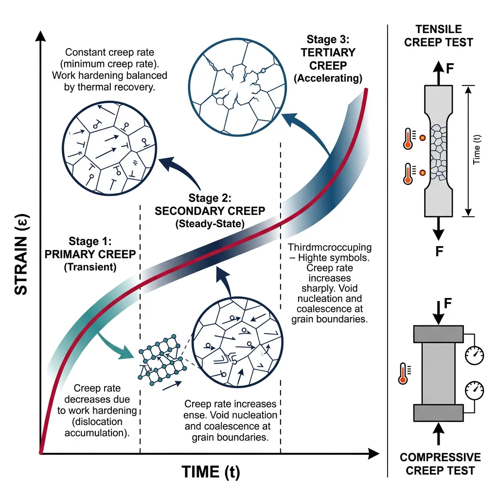
A standard creep test applies constant load to a specimen at constant temperature and records strain vs. time. The resulting creep curve has three stages:
- Primary Creep (Stage I): Decreasing creep rate — strain hardening dominates. Dislocations accumulate and tangles form, making further deformation progressively harder. Think: pushing through a crowd that's getting denser.
- Secondary (Steady-State) Creep (Stage II): Constant creep rate — a dynamic balance between strain hardening and thermal recovery. This regime dominates the component's service life and is the basis for engineering design. The steady-state creep rate follows the Arrhenius equation: $\dot{\varepsilon}_s = A\sigma^n e^{-Q_c/RT}$ where $n$ is the stress exponent and $Q_c$ is the activation energy for the rate-controlling creep mechanism.
- Tertiary Creep (Stage III): Accelerating creep rate — internal damage accumulates (void nucleation at grain boundaries, necking, microstructural degradation). Ends in creep rupture.
- Low T (0.4–0.5 T_m): Dislocation glide — stress exponent $n ≈ 3$–$5$ (power-law creep)
- Intermediate T (0.5–0.7 T_m): Dislocation climb — vacancies allow dislocations to bypass obstacles, $n ≈ 4$–$6$
- High T, low σ (>0.7 T_m): Diffusion creep — atoms flow along grain boundaries (Coble creep, $n = 1$) or through the lattice (Nabarro-Herring creep, $n = 1$)
- High T, high σ: Grain boundary sliding — grains slide past each other, often combining with diffusion mechanisms
Stress Rupture & Larson-Miller
Engineers designing jet engine turbine blades need to predict how long a component will last under specific stress and temperature combinations. Creep testing to actual service lives (tens of thousands of hours) is impractical, so engineers use time-temperature parametrization — short-term tests at higher temperatures to predict long-term behavior at lower temperatures.
The most widely used approach is the Larson-Miller parameter (LMP):
$$LMP = T(C + \log_{10} t_r)$$where $T$ is temperature in Kelvin (or Rankine), $t_r$ is time to rupture in hours, and $C$ is a material constant (typically 20 for most alloys). The power of this approach is that for a given material and stress, the LMP is constant — trading time for temperature. A component that lasts 100,000 hours at 800 °C might be equivalent to one tested at 900 °C for only 1,000 hours.
Case Study: Jet Engine Turbine Blade Creep
Modern jet engine high-pressure turbine blades operate at gas temperatures up to 1,500 °C — above the melting point of the nickel superalloy from which they're made (~1,350 °C). This is only possible through internal cooling passages, thermal barrier coatings (TBC), and single-crystal casting:
- Internal cooling channels: Labyrinthine passages carry compressed bleed air through the blade interior, reducing metal temperature by 200–300 °C
- Thermal barrier coating: A 100–300 μm layer of yttria-stabilized zirconia (YSZ) provides a further 100–150 °C temperature drop at the metal surface
- Single-crystal casting: Eliminating grain boundaries removes the primary creep failure mechanism (grain boundary sliding). Single-crystal CMSX-4 superalloy has 10× greater creep life than conventionally cast equivalents
- Precipitate strengthening: 70% volume fraction of γ′ (Ni₃Al) precipitates, coherent with the γ matrix, blocks dislocation motion up to ~1,050 °C
Design life: These blades must withstand centrifugal stresses of ~150 MPa at ~1,050 °C metal temperature for 20,000+ flight hours. The Larson-Miller parameter guides inspection intervals and retirement-for-cause criteria.
import numpy as np
import matplotlib.pyplot as plt

# Larson-Miller parameter calculations for creep life prediction
# Material: Inconel 718 nickel superalloy

C_LM = 20  # Larson-Miller constant (typical value)

def larson_miller(T_celsius, t_rupture_hours):
    """Calculate Larson-Miller parameter"""
    T_kelvin = T_celsius + 273.15
    return T_kelvin * (C_LM + np.log10(t_rupture_hours))

def predict_rupture_time(T_celsius, LMP):
    """Predict rupture time from LMP and temperature"""
    T_kelvin = T_celsius + 273.15
    log_tr = LMP / T_kelvin - C_LM
    return 10 ** log_tr  # hours

# Example: Test data at accelerated (high-temperature) condition
T_test = 750  # °C (accelerated test temperature)
t_test = 500  # hours to rupture in accelerated test
stress = 300  # MPa

LMP_value = larson_miller(T_test, t_test)
print(f"=== Larson-Miller Creep Life Prediction ===")
print(f"Stress: {stress} MPa")
print(f"Test condition: {T_test}°C, ruptured at {t_test} hours")
print(f"Larson-Miller Parameter: {LMP_value:.0f}")

# Predict life at service temperature
T_service = 650  # °C (actual service temperature)
t_service = predict_rupture_time(T_service, LMP_value)
print(f"\nPredicted rupture time at {T_service}°C: {t_service:,.0f} hours")
print(f"  = {t_service/8760:.1f} years of continuous operation")
print(f"  = {t_service/4000:.1f} years at 4000 flight-hours/year")

# Plot LMP diagram — rupture time vs temperature for a fixed stress
temps = np.linspace(550, 850, 200)
times = predict_rupture_time(temps, LMP_value)

plt.figure(figsize=(10, 5))
plt.semilogy(temps, times, 'b-', linewidth=2)
plt.axhline(y=20000, color='r', linestyle='--', alpha=0.7, label='Design life = 20,000 hrs')
plt.axvline(x=T_service, color='g', linestyle=':', alpha=0.7, label=f'Service temp = {T_service}°C')
plt.scatter([T_test], [t_test], color='red', s=100, zorder=5, label=f'Test point ({T_test}°C, {t_test} hrs)')
plt.xlabel('Temperature (°C)', fontsize=12)
plt.ylabel('Rupture Time (hours)', fontsize=12)
plt.title(f'Creep Rupture Life vs Temperature — σ = {stress} MPa (Inconel 718)', fontsize=13)
plt.legend(fontsize=10)
plt.grid(True, alpha=0.3, which='both')
plt.ylim(1, 1e7)
plt.tight_layout()
plt.show()
In-Situ & Advanced Testing
Modern materials development demands more than simple pass/fail testing — engineers need to watch how materials deform at the microstructural level, in real time, under realistic conditions. Several advanced techniques have transformed mechanical characterization:
Digital Image Correlation (DIC): A camera-based technique that tracks a speckle pattern painted on the specimen surface to measure full-field displacement and strain maps with sub-pixel resolution. Unlike a strain gauge (one point), DIC reveals the complete strain distribution — showing strain localization, shear bands, and neck formation as they evolve. Think of it as a "strain movie" of the entire specimen surface.
In-Situ SEM/TEM Testing: Miniaturized testing stages mounted inside scanning or transmission electron microscopes allow researchers to observe dislocation motion, crack nucleation, and phase transformations as they happen during deformation. These experiments directly connect macroscopic stress-strain behavior to the underlying microstructural mechanisms — something that was pure inference just decades ago.
High-Throughput Mechanical Testing: Combinatorial approaches borrow ideas from pharmaceutical screening: create a library of compositions or microstructures on a single sample (using gradient sputtering, diffusion multiples, or additive manufacturing) and rapidly test hundreds of conditions using automated nanoindentation arrays. This accelerates the traditional alloy development cycle from years to weeks.
Mechanical Properties Report Generator
Use this interactive tool to generate a formatted mechanical properties test report. Enter your test data below and download as a Word document, Excel spreadsheet, or PDF report.
Mechanical Properties Report Generator
Enter test parameters and measured values. Download as Word, Excel, or PDF.
All data stays in your browser. Nothing is sent to or stored on any server.
Exercises & Practice Problems
- Stress-Strain Analysis: A cylindrical steel specimen (diameter = 12.8 mm, gauge length = 50.8 mm) is subjected to a tensile test. At a load of 54.2 kN, the gauge length has increased to 50.95 mm. (a) Calculate the engineering stress and strain. (b) If the Young's modulus is 207 GPa, is this deformation elastic or plastic? (c) Calculate the true stress and true strain at this point.
- Elastic Moduli Relationships: A material has a Young's modulus of 310 GPa and a Poisson's ratio of 0.30. (a) Calculate the shear modulus. (b) Calculate the bulk modulus. (c) If a 2 m long bar of this material is loaded with 50 kN along its 20 mm × 20 mm cross-section, how much does it elongate? How much does the cross-section contract laterally?
- Hardness Correlation: A Brinell hardness test on a low-carbon steel sample yields HB 180. (a) Estimate the ultimate tensile strength using the empirical correlation. (b) If another specimen of the same steel has HRC 25 after heat treatment, which specimen is harder? Use the conversion relationships to compare.
- Fatigue Design (Goodman): A component made from a steel with $\sigma_{UTS}$ = 800 MPa and endurance limit $S_e$ = 350 MPa is subjected to cyclic loading with a mean stress of 200 MPa. Using the Goodman criterion, what is the maximum allowable stress amplitude for infinite life?
- Fracture Mechanics: An edge crack of length 3 mm is detected in a large plate of 7075-T6 aluminum ($K_{IC}$ = 27 MPa√m). Using $Y$ = 1.12 for an edge crack, (a) what is the maximum stress that can be applied without fracture? (b) If the service stress is 150 MPa, what is the critical crack length?
- Creep Life Prediction: A nickel superalloy turbine blade is tested at 850 °C and ruptures after 200 hours at a stress of 250 MPa. Using $C$ = 20 for the Larson-Miller parameter, (a) calculate the LMP. (b) Predict the rupture time at the actual service temperature of 750 °C at the same stress. (c) If a 10,000-hour service life is required, what is the maximum allowable service temperature?
Conclusion & Next Steps
Mechanical behavior and testing form the critical bridge between materials science and engineering design. We've journeyed from the fundamental stress-strain curve — the fingerprint of every material — through hardness testing methods that provide rapid quality control, fatigue analysis that prevents 90% of mechanical failures, fracture mechanics that sizes cracks before they become catastrophic, and creep behavior that governs high-temperature design life. Every concept connects: the elastic modulus governs stiffness, the yield strength sets design limits, the fracture toughness determines damage tolerance, and the Larson-Miller parameter enables safe high-temperature operation. Together, these properties and testing methods form the language engineers use to select materials, predict performance, and prevent failure.