Materials Science & Engineering Series Part 10: Thermodynamics & Kinetics of Materials

Thermodynamic Foundations

Thermodynamics and kinetics are the twin pillars that govern every material transformation. Thermodynamics tells us whether a reaction or transformation is energetically favorable — it defines the destination. Kinetics tells us how fast we get there and by what pathway. Together, they dictate everything from how steel is hardened to how silicon crystals are grown for semiconductors.

The three laws of thermodynamics underpin all of materials science:

• First Law (energy conservation): Energy is neither created nor destroyed — it only changes form. The internal energy change equals heat added minus work done: dU = δQ − δW.
• Second Law (entropy): The total entropy of an isolated system always increases. Spontaneous processes move toward states of higher disorder. This is why alloys mix, why ice melts at room temperature, and why diffusion proceeds from high to low concentration.
• Third Law: The entropy of a perfect crystal approaches zero as temperature approaches absolute zero, providing a reference point for entropy calculations.

Gibbs Free Energy & Chemical Potential

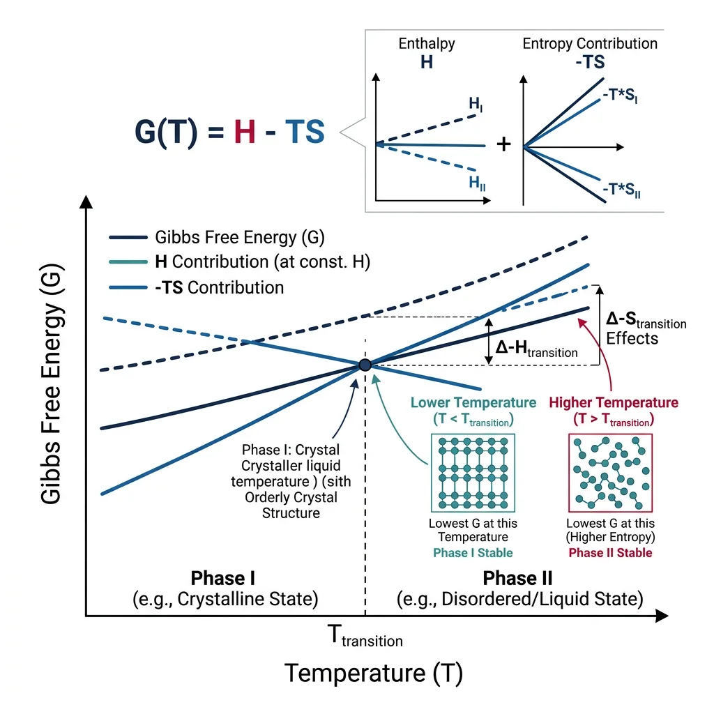
The most powerful thermodynamic quantity for materials engineering is the Gibbs free energy:

The chemical potential μ_i of component i is the partial molar Gibbs energy — it measures how much the total free energy changes when you add an infinitesimal amount of species i: μ_i = (∂G/∂n_i)_T,P,nj≠i. At equilibrium, the chemical potential of each component is equal in all coexisting phases.

Activity (a) quantifies the "effective concentration" of a component, accounting for non-ideal interactions: μ_i = μ_i° + RT·ln(a_i). For an ideal solution, activity equals mole fraction (a_i = x_i). For real solutions, a_i = γ_i·x_i, where γ is the activity coefficient capturing intermolecular interactions.

Python: Gibbs Free Energy of Mixing vs. Composition

import numpy as np
import matplotlib.pyplot as plt

# Gibbs free energy of mixing for an ideal binary solution
# G_mix = RT * [x*ln(x) + (1-x)*ln(1-x)]
R = 8.314  # J/(mol·K)
temperatures = [500, 1000, 1500, 2000]  # Kelvin
x = np.linspace(0.001, 0.999, 500)  # mole fraction of component B

plt.figure(figsize=(10, 6))
for T in temperatures:
    G_mix = R * T * (x * np.log(x) + (1 - x) * np.log(1 - x))
    plt.plot(x, G_mix / 1000, label=f'T = {T} K', linewidth=2)

plt.xlabel('Mole Fraction of B (x_B)', fontsize=12)
plt.ylabel('ΔG_mix (kJ/mol)', fontsize=12)
plt.title('Gibbs Free Energy of Ideal Mixing', fontsize=14)
plt.legend(fontsize=11)
plt.grid(True, alpha=0.3)
plt.axhline(y=0, color='black', linewidth=0.5)
plt.tight_layout()
plt.show()

# Key insight: G_mix is always negative for ideal mixing
# (mixing is always spontaneous), and the minimum deepens
# with temperature because the -TS term dominates.
print("At T=1000K, minimum G_mix =", round(R * 1000 * (0.5 * np.log(0.5) + 0.5 * np.log(0.5)) / 1000, 2), "kJ/mol")

Phase Equilibria & Phase Rules

The Gibbs Phase Rule defines the degrees of freedom F (number of independently variable intensive properties) for a system in equilibrium:

Key binary phase diagram types:

• Eutectic (e.g., Pb-Sn): Liquid → α + β simultaneously at the eutectic temperature. The microstructure shows a characteristic lamellar or rod-like two-phase mixture. Solder alloys exploit the low eutectic melting point.
• Peritectic (e.g., Fe-C at 1493°C): Liquid + δ → γ. A solid phase reacts with liquid to form a different solid phase. Common in steels and many intermetallic systems.
• Eutectoid (e.g., Fe-C at 727°C): γ → α + Fe₃C. A single solid transforms to two new solids — the foundation of steel heat treatment. Pearlite (lamellar α + cementite) forms from austenite at this temperature.

Phase Equilibria & Computational Thermodynamics

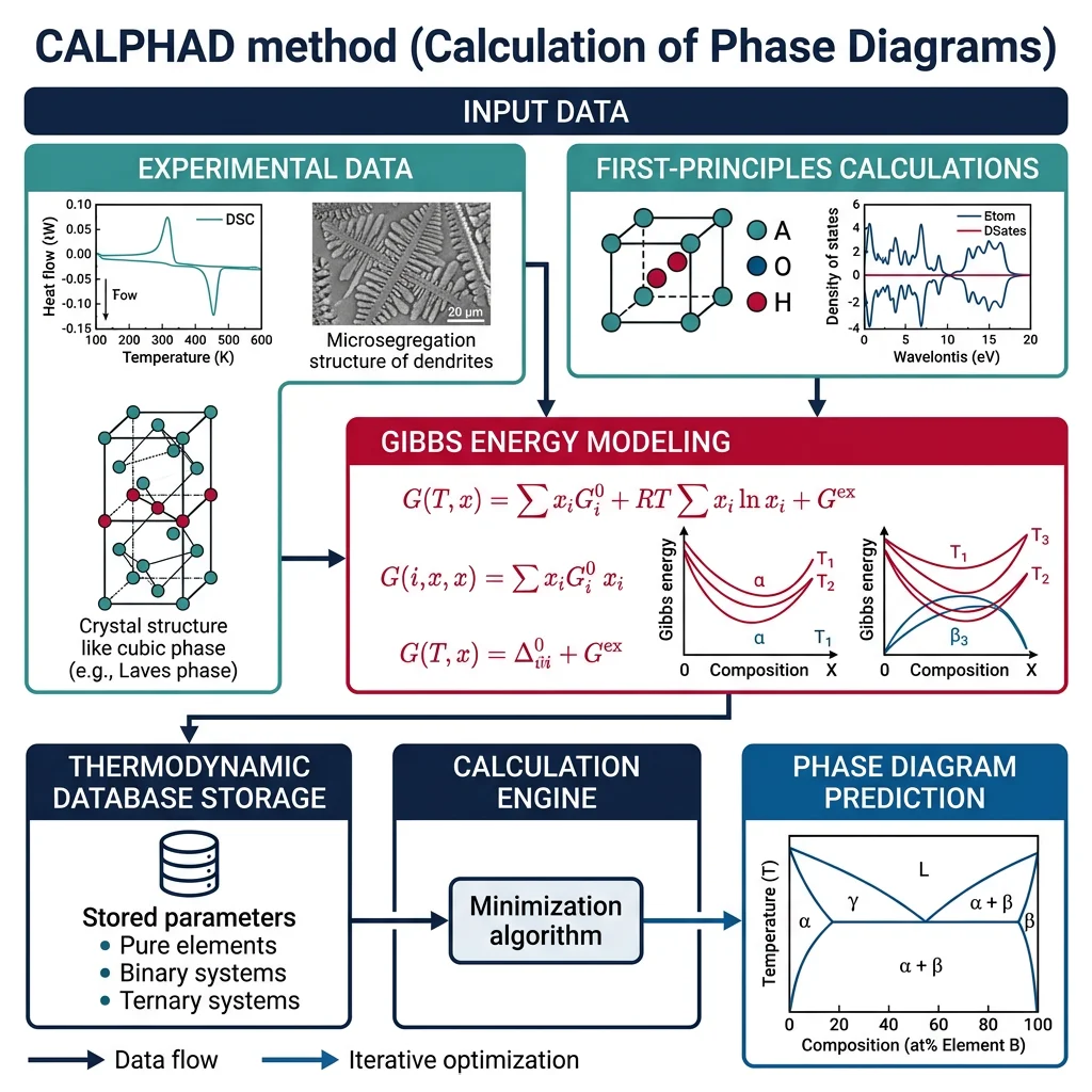
The CALPHAD method (CALculation of PHAse Diagrams) is the workhorse of modern alloy design. Rather than measuring every possible alloy composition experimentally, CALPHAD uses thermodynamic models fitted to known data points to predict phase stability across the entire composition-temperature space.

Solution Models & Activity

CALPHAD relies on mathematical models for the Gibbs energy of each phase:

• Ideal Solution: G_mix = RT Σ x_i ln(x_i). Assumes atoms mix randomly with no preferential interactions. Good for similar elements (e.g., Cu-Ni).
• Regular Solution: G_mix = RT Σ x_i ln(x_i) + Ω·x_A·x_B. Adds one interaction parameter Ω. If Ω > 0 (repulsive), the system tends to unmix (miscibility gap). If Ω < 0 (attractive), ordering or compound formation is favored.
• Redlich-Kister Polynomials: G^excess = x_Ax_B Σ L_ν(x_A − x_B)^ν, where L_ν are temperature-dependent parameters. This flexible form captures asymmetric interactions and is the standard in CALPHAD databases.
• Sub-lattice Models: For ordered phases (intermetallics, carbides), atoms occupy specific crystallographic sites. The Compound Energy Formalism (CEF) models each sub-lattice independently — essential for phases like Ni₃Al (γ′) in superalloys.

Multicomponent Phase Diagrams

Real engineering alloys contain 5–15 elements. CALPHAD's power lies in extrapolating binary and ternary assessments to multicomponent systems — the pairwise interaction parameters combine to predict behavior in complex alloys that would be impossible to map experimentally.

Python: Binary Phase Diagram Construction (Regular Solution)

import numpy as np
import matplotlib.pyplot as plt

# Construct a binary eutectic phase diagram using regular solution model
# Two solid phases (alpha, beta) with limited solubility
R = 8.314  # J/(mol·K)
T_mA = 1000  # Melting point of pure A (K)
T_mB = 800   # Melting point of pure B (K)
L_A = 12000  # Latent heat of fusion A (J/mol)
L_B = 9000   # Latent heat of fusion B (J/mol)
Omega_s = 20000  # Interaction parameter in solid (positive = demixing)
Omega_l = 5000   # Interaction parameter in liquid

# Calculate liquidus and solidus using equal chemical potential condition
T_range = np.linspace(400, 1050, 500)

# For each temperature, find compositions where G_solid = G_liquid
# Simplified: use tangent construction approach
x_liquidus_A = []  # liquidus from A-rich side
x_solidus_A = []   # solidus from A-rich side
T_plot = []

for T in T_range:
    # Free energy difference (liquid - solid) for pure components
    dG_A = L_A * (1 - T / T_mA)  # positive below T_mA (solid stable)
    dG_B = L_B * (1 - T / T_mB)
    
    # Scan compositions to find phase boundaries
    x = np.linspace(0.001, 0.999, 2000)
    G_solid = R * T * (x * np.log(x) + (1-x) * np.log(1-x)) + Omega_s * x * (1-x)
    G_liquid = R * T * (x * np.log(x) + (1-x) * np.log(1-x)) + Omega_l * x * (1-x) - (1-x)*dG_A - x*dG_B
    
    dG = G_liquid - G_solid
    # Find zero crossings (phase boundaries)
    crossings = np.where(np.diff(np.sign(dG)))[0]
    if len(crossings) >= 2:
        T_plot.append(T)
        x_liquidus_A.append(x[crossings[0]])
        x_solidus_A.append(x[crossings[1]])

plt.figure(figsize=(10, 7))
plt.fill_betweenx(T_plot, x_liquidus_A, x_solidus_A, alpha=0.3, color='coral', label='Two-phase (L+S)')
plt.plot(x_liquidus_A, T_plot, 'r-', linewidth=2, label='Liquidus')
plt.plot(x_solidus_A, T_plot, 'b-', linewidth=2, label='Solidus')
plt.xlabel('Mole Fraction of B', fontsize=12)
plt.ylabel('Temperature (K)', fontsize=12)
plt.title('Binary Phase Diagram (Regular Solution Model)', fontsize=14)
plt.legend(fontsize=11)
plt.grid(True, alpha=0.3)
plt.xlim(0, 1)
plt.tight_layout()
plt.show()
print("Phase diagram constructed with Omega_solid =", Omega_s, "J/mol")
print("Positive Omega in solid promotes phase separation (eutectic behavior)")

Kinetics & Phase Transformations

While thermodynamics predicts the equilibrium destination, kinetics governs the journey — how fast atoms rearrange, how new phases nucleate and grow, and how processing conditions (heating rate, cooling rate, hold time) control the final microstructure.

Nucleation Theory

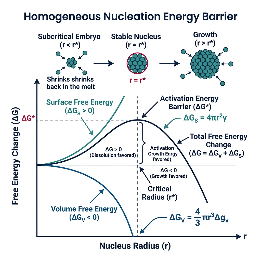
Every phase transformation begins with nucleation — the formation of tiny embryos of the new phase within the parent phase. Nucleation requires overcoming an energy barrier because creating a new interface costs energy.

Homogeneous nucleation occurs uniformly throughout the bulk material. The total free energy change for forming a spherical nucleus of radius r is: ΔG = −(4/3)πr³·ΔG_v + 4πr²·γ, where ΔG_v is the volume free energy driving force (energy gained) and γ is the interfacial energy (energy cost). The critical radius r* = 2γ/ΔG_v — nuclei smaller than r* shrink and dissolve; larger ones grow spontaneously.

Heterogeneous nucleation occurs preferentially at defects — grain boundaries, dislocations, free surfaces, inclusions — because these sites reduce the interfacial energy cost. The activation barrier is reduced by a factor f(θ) = (2 + cosθ)(1 − cosθ)²/4, where θ is the contact angle. In practice, nearly all real transformations nucleate heterogeneously — that's why grain refiners and inoculants are added to control nucleation sites.

TTT & CCT Diagrams

TTT (Time-Temperature-Transformation) diagrams map when phase transformations begin and end during isothermal holds. They have a characteristic "C-curve" shape because:

• At high temperatures (just below equilibrium): large thermodynamic driving force is low → slow nucleation → transformation takes long.
• At low temperatures: high driving force but atomic mobility is limited → slow diffusion → transformation again takes long.
• At intermediate temperatures: optimal balance of driving force and diffusivity → fastest transformation → the "nose" of the C-curve.

CCT (Continuous Cooling Transformation) diagrams are the practical counterpart — they show what happens during continuous cooling at different rates, which is what actually occurs in heat treatment. CCT curves are shifted to longer times and lower temperatures compared to TTT curves because the transformation has less time to proceed at each temperature.

Avrami Kinetics & Coarsening

The Avrami equation (also Johnson-Mehl-Avrami-Kolmogorov, JMAK) describes the fraction of material transformed over time during isothermal phase transformations:

The characteristic S-shaped (sigmoidal) curve of the Avrami equation captures three stages: (1) an incubation period with slow initial transformation, (2) rapid acceleration as growing nuclei impinge on untransformed volume, and (3) saturation as the matrix is consumed. The parameter k follows an Arrhenius relationship: k = k₀·exp(−Q/RT), where Q is the activation energy for the transformation.

Python: Avrami Kinetics Simulation

import numpy as np
import matplotlib.pyplot as plt

# Avrami equation: f(t) = 1 - exp(-k * t^n)
# Simulate for different Avrami exponents
t = np.linspace(0, 10, 500)  # time (arbitrary units)
k = 0.01  # rate constant

avrami_exponents = [1, 2, 3, 4]
labels = [
    'n=1 (1D thickening)',
    'n=2 (2D growth, no nucleation)',
    'n=3 (3D growth, site-saturated)',
    'n=4 (3D growth, constant nucleation)'
]

plt.figure(figsize=(10, 6))
for n, label in zip(avrami_exponents, labels):
    f = 1 - np.exp(-k * t**n)
    plt.plot(t, f, linewidth=2, label=label)

plt.xlabel('Time (arbitrary units)', fontsize=12)
plt.ylabel('Fraction Transformed, f(t)', fontsize=12)
plt.title('Avrami Kinetics: Effect of Exponent n', fontsize=14)
plt.legend(fontsize=10)
plt.grid(True, alpha=0.3)
plt.ylim(0, 1.05)
plt.tight_layout()
plt.show()

# Determine time to 50% transformation for each n
for n, label in zip(avrami_exponents, labels):
    t_half = (np.log(2) / k) ** (1/n)
    print(f"{label}: t_50% = {t_half:.2f}")

Solidification & Diffusion

Solidification — the transformation from liquid to solid — is the starting point for most metallic components. Understanding solidification thermodynamics and kinetics is critical for controlling casting microstructures, avoiding defects, and achieving desired properties.

Solidification Fundamentals

Nucleation in solidification follows the same principles as solid-state nucleation: undercooling below the equilibrium melting point provides the thermodynamic driving force, while the solid-liquid interfacial energy creates the nucleation barrier. Heterogeneous nucleation on mold walls, inoculant particles, or oxide inclusions dominates in practice — typical undercoolings in industrial casting are only 1–10°C, versus hundreds of degrees for homogeneous nucleation.

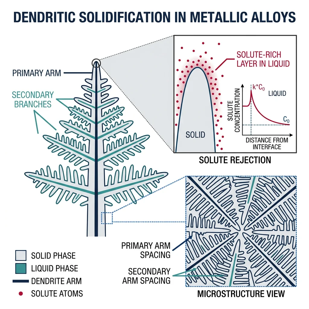
Dendritic growth is the most common solidification morphology. As a solid nucleus grows into the undercooled liquid, it develops tree-like branching structures (dendrites) because perturbations at the solid-liquid interface grow faster than the flat interface — this is the Mullins-Sekerka instability. Primary arms grow along preferred crystallographic directions (⟨100⟩ in cubic crystals), with secondary and tertiary branches filling the space between.

Diffusion & Fick's Laws

Diffusion — the thermally activated movement of atoms through a material — underlies virtually every kinetic process in materials science: phase transformations, homogenization, oxidation, creep, and sintering.

Fick's First Law (steady-state): J = −D·(dC/dx), where J is the flux (atoms/m²·s), D is the diffusivity (m²/s), and dC/dx is the concentration gradient. The negative sign indicates atoms move from high to low concentration — downhill on the chemical potential landscape.

Fick's Second Law (non-steady-state): ∂C/∂t = D·(∂²C/∂x²). This partial differential equation describes how concentration profiles evolve over time and is the workhorse equation for most diffusion problems in materials processing.

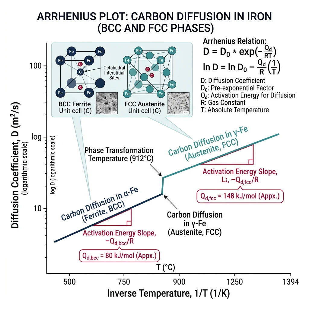
The diffusion coefficient follows an Arrhenius relationship: D = D₀·exp(−Q_d/RT), where D₀ is the pre-exponential factor and Q_d is the activation energy. Typical values for carbon in FCC iron (austenite): D₀ ≈ 2.3×10⁻⁵ m²/s, Q_d ≈ 148 kJ/mol — giving D ≈ 10⁻¹¹ m²/s at 1000°C.

Carburizing & Diffusion Simulation

Python: Diffusion Profile — Fick's Second Law with Error Function

import numpy as np
import matplotlib.pyplot as plt
from scipy.special import erf

# Carburizing simulation: Fick's second law solution
# C(x,t) = Cs - (Cs - C0) * erf(x / (2*sqrt(D*t)))
Cs = 0.80   # surface carbon concentration (wt%)
C0 = 0.20   # initial carbon concentration (wt%)
D = 1.28e-11  # diffusivity of C in austenite at 925°C (m²/s)

# Distance from surface
x = np.linspace(0, 3e-3, 500)  # 0 to 3 mm in meters

# Different carburizing times
times_hours = [2, 4, 8, 12, 16]  # hours

plt.figure(figsize=(10, 6))
for t_hr in times_hours:
    t = t_hr * 3600  # convert to seconds
    C = Cs - (Cs - C0) * erf(x / (2 * np.sqrt(D * t)))
    plt.plot(x * 1000, C, linewidth=2, label=f't = {t_hr} hrs')

# Mark the 0.40%C case depth threshold
plt.axhline(y=0.40, color='red', linestyle='--', alpha=0.7, label='Case depth threshold (0.40%C)')

plt.xlabel('Distance from Surface (mm)', fontsize=12)
plt.ylabel('Carbon Concentration (wt%)', fontsize=12)
plt.title('Carburizing Diffusion Profiles at 925°C', fontsize=14)
plt.legend(fontsize=10)
plt.grid(True, alpha=0.3)
plt.ylim(0.15, 0.85)
plt.tight_layout()
plt.show()

# Calculate case depth (x at C=0.40) for each time
print("Case depths at C = 0.40 wt%C:")
for t_hr in times_hours:
    t = t_hr * 3600
    # erf(z) = (Cs - 0.40) / (Cs - C0) = 0.667, z ≈ 0.685
    z = 0.685
    case_depth_mm = 2 * z * np.sqrt(D * t) * 1000
    print(f"  t = {t_hr:2d} hrs → case depth = {case_depth_mm:.2f} mm")

Practice Exercises

Conclusion & Next Steps

Thermodynamics and kinetics form the quantitative backbone of materials science and engineering. With Gibbs free energy and chemical potential, we predict which phases are stable. With CALPHAD, we computationally explore vast composition spaces that would take lifetimes to map experimentally. With nucleation theory and the Avrami equation, we understand how and how fast transformations proceed. With Fick's laws and TTT/CCT diagrams, we design heat treatments and processing schedules that deliver precisely controlled microstructures.

The interplay between thermodynamic driving forces and kinetic barriers is what makes materials processing both an art and a science — the same alloy can become soft or hard, brittle or tough, simply by controlling the thermal pathway. Mastering these concepts empowers you to not only understand existing materials but to design new ones for the challenges ahead.