Iron-Carbon System & Steels
Materials Science Mastery
Atomic Structure & Quantum Foundations
Quantum mechanics, bonding, band theory, Fermi energy, phononsCrystal Structures, Defects & Diffusion
FCC/BCC/HCP, Miller indices, dislocations, phase diagrams, Fick's lawsMetals & Alloys
Iron-carbon diagram, steels, aluminum, titanium, superalloys, heat treatmentPolymers & Soft Materials
Polymer chemistry, thermoplastics, viscoelasticity, rheology, biopolymersCeramics, Glass & Composites
Oxide ceramics, toughening, fiber-reinforced composites, interfacial bondingMechanical Behavior & Testing
Stress-strain, hardness, fatigue, fracture toughness, nanoindentationFailure Analysis & Reliability Engineering
Fractography, corrosion, tribology, root cause analysisNanomaterials & Smart Materials
Nanotubes, graphene, piezoelectrics, shape memory alloys, self-healingMaterials Characterization Techniques
XRD, SEM, TEM, AFM, DSC, TGA, spectroscopyThermodynamics & Kinetics of Materials
Gibbs free energy, CALPHAD, phase stability, solidificationElectronic, Magnetic & Optical Materials
Semiconductors, photovoltaics, dielectrics, superconductorsBiomaterials
Implants, biocompatibility, tissue engineering, drug deliveryEnergy Materials
Battery materials, hydrogen storage, fuel cells, nuclear materialsComputational Materials Science
DFT, molecular dynamics, FEM, materials informatics, AIThink of the iron-carbon phase diagram as a GPS for metallurgists — a map that tells you exactly what microstructure you'll get for any combination of carbon content (x-axis) and temperature (y-axis). Just as a recipe tells you what happens when you bake flour and sugar at different temperatures, the iron-carbon diagram tells you what happens when you heat or cool iron with different amounts of carbon.
Iron is remarkable because it undergoes allotropic transformations — it changes its crystal structure at different temperatures even in its pure form. At room temperature, pure iron is BCC (body-centered cubic), called α-ferrite. Heat it to 912°C and it transforms to FCC (face-centered cubic), called γ-austenite. Heat further to 1394°C and it reverts to BCC, called δ-ferrite, before melting at 1538°C.
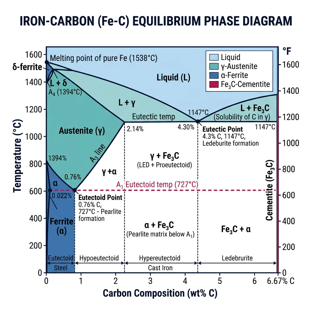
- α-Ferrite: BCC iron with very limited carbon solubility (max 0.022 wt% C at 727°C). Soft, ductile, magnetic. The matrix phase of most steels at room temperature.
- γ-Austenite: FCC iron that dissolves up to 2.14 wt% C at 1147°C. Non-magnetic. The high-temperature phase where most heat treatments begin.
- Cementite (Fe₃C): An intermetallic compound with 6.67 wt% C. Extremely hard and brittle. Acts as a reinforcing phase in steels.
- Pearlite: A lamellar (layered) mixture of ferrite and cementite. Forms at 727°C. Looks like a fingerprint under the microscope — alternating bright (ferrite) and dark (cementite) layers.
- Martensite: A supersaturated, body-centered tetragonal (BCT) phase formed by rapid quenching of austenite. Extremely hard but brittle — the basis of hardened steels.
The two most critical reactions on the diagram are:
- Eutectoid Reaction (727°C, 0.76 wt% C): Austenite → Ferrite + Cementite (γ → α + Fe₃C). This produces pearlite. Think of it as "one solid splitting into two solids."
- Eutectic Reaction (1147°C, 4.3 wt% C): Liquid → Austenite + Cementite (L → γ + Fe₃C). This produces a structure called ledeburite and defines the boundary between steels (<2.14% C) and cast irons (>2.14% C).
Analogy — The Freezing Lake: Just as a lake has a shoreline that separates water from land, and the exact shape of that shoreline changes with the seasons, the iron-carbon diagram has boundary lines that separate different phases. Above certain lines, atoms are mobile and dissolved (like water); below them, atoms are locked into ordered structures (like ice). Where you are on the map tells you exactly what "landscape" of phases you're standing in.
import numpy as np
import matplotlib.pyplot as plt
import matplotlib.patches as mpatches

# Simplified Iron-Carbon Phase Diagram (up to 6.67 wt% C)
fig, ax = plt.subplots(figsize=(12, 8))

# Key boundary lines (simplified)
# Liquidus line
c_liq = [0, 0.76, 2.14, 4.3, 6.67]
t_liq = [1538, 1493, 1495, 1147, 1147]
ax.plot(c_liq[:3], t_liq[:3], 'r-', linewidth=2, label='Liquidus')
ax.plot(c_liq[2:], t_liq[2:], 'r-', linewidth=2)

# A3 line (ferrite-austenite boundary)
c_a3 = [0, 0.022, 0.76]
t_a3 = [912, 727, 727]
ax.plot(c_a3, t_a3, 'b-', linewidth=2, label='A3 line')

# Acm line (austenite-cementite boundary)
c_acm = [0.76, 2.14]
t_acm = [727, 1147]
ax.plot(c_acm, t_acm, 'g-', linewidth=2, label='Acm line')

# Eutectoid isotherm
ax.axhline(y=727, color='purple', linestyle='--', linewidth=1.5, label='Eutectoid (727°C)')

# Eutectic isotherm
ax.axhline(y=1147, xmin=2.14/7, xmax=1.0, color='orange',
           linestyle='--', linewidth=1.5, label='Eutectic (1147°C)')

# Mark critical points
points = {'Eutectoid': (0.76, 727), 'Eutectic': (4.3, 1147)}
for name, (cx, ty) in points.items():
    ax.plot(cx, ty, 'ko', markersize=8)
    ax.annotate(name, (cx, ty), textcoords="offset points",
                xytext=(10, 10), fontsize=10, fontweight='bold')

# Phase region labels
ax.text(0.3, 1100, 'γ\n(Austenite)', fontsize=14, ha='center',
        fontweight='bold', color='navy')
ax.text(0.1, 500, 'α\n(Ferrite)', fontsize=12, ha='center',
        fontweight='bold', color='blue')
ax.text(1.0, 400, 'α + Fe₃C\n(Pearlite\nregion)', fontsize=10,
        ha='center', color='purple')
ax.text(0.5, 1400, 'Liquid', fontsize=14, ha='center',
        fontweight='bold', color='red')

# Formatting
ax.set_xlabel('Carbon Content (wt%)', fontsize=13, fontweight='bold')
ax.set_ylabel('Temperature (°C)', fontsize=13, fontweight='bold')
ax.set_title('Simplified Iron-Carbon Phase Diagram', fontsize=15,
             fontweight='bold')
ax.set_xlim(0, 6.67)
ax.set_ylim(200, 1600)
ax.axvline(x=2.14, color='gray', linestyle=':', alpha=0.5)
ax.text(2.14, 250, '2.14%\nSteel | Cast Iron', ha='center',
        fontsize=9, color='gray')
ax.legend(loc='upper right', fontsize=9)
ax.grid(True, alpha=0.3)
plt.tight_layout()
plt.show()
The Eutectoid Reaction — How Pearlite Forms
Imagine cooling a steel with exactly 0.76 wt% carbon (a eutectoid steel) slowly from 800°C. Above 727°C, the entire microstructure is uniform austenite — carbon atoms happily dissolved in the FCC lattice. As the temperature crosses 727°C, something dramatic happens: the austenite becomes thermodynamically unstable and begins to decompose. Carbon atoms, which were uniformly distributed, start clustering together to form carbon-rich cementite (Fe₃C) plates, leaving behind carbon-depleted ferrite (α) between them.
The result is pearlite — alternating lamellae of soft ferrite and hard cementite, named because its iridescent appearance under the microscope resembles mother-of-pearl. The spacing of these lamellae depends on cooling rate: slow cooling produces coarse pearlite (widely spaced, softer, ~200 HV), while faster cooling produces fine pearlite (tightly spaced, harder, ~300 HV). If you cool fast enough to skip pearlite formation entirely, you get martensite — which we'll explore in the heat treatment section.
Steel Classifications
Steels are classified primarily by their carbon content, which determines their balance of strength, ductility, and weldability. Think of carbon as a "stiffener" — the more you add, the harder and stronger the steel becomes, but it also becomes more brittle and harder to weld.
- Low Carbon / Mild Steel (<0.25% C): Highly ductile, easily welded and formed. Used for structural beams (I-beams), automotive body panels, nails, wire, and sheet metal. Yield strength: 200–350 MPa. The workhorse of construction.
- Medium Carbon Steel (0.25–0.60% C): Balanced strength and ductility. Can be heat-treated (quenched and tempered) for improved properties. Used for axles, crankshafts, gears, railway tracks, and forged components. Yield strength: 350–600 MPa.
- High Carbon Steel (0.60–1.4% C): Very hard but brittle. Always heat-treated for use. Springs, cutting tools, piano wire, razor blades, chisels. Yield strength: 500–1000+ MPa but with reduced ductility (<10% elongation).
- Cast Iron (>2.14% C): Technically not steel. Contains graphite flakes (gray iron) or nodules (ductile iron). Excellent castability and vibration damping. Used for engine blocks, pipes, manhole covers.
The AISI/SAE designation system uses a four-digit code where the first two digits indicate the alloy type and the last two give the carbon content in hundredths of a percent. For example:
- AISI 1020: 10xx = plain carbon steel, 20 = 0.20% carbon → low carbon structural steel
- AISI 1045: Plain carbon steel with 0.45% C → medium carbon, used for shafts and gears
- AISI 4140: 41xx = Cr-Mo alloy steel, 40 = 0.40% C → a premium general-purpose alloy steel
- AISI 4340: Ni-Cr-Mo alloy steel with 0.40% C → high-strength aircraft landing gear steel
| Application | Recommended Grade | Why? |
|---|---|---|
| Building frames, bridges | ASTM A36 (0.25% C max) | Excellent weldability, low cost |
| Car gears, crankshafts | AISI 4140 | Hardenable, tough, fatigue-resistant |
| Springs, lock washers | AISI 1095 | High hardness after heat treatment |
| Drill bits, saw blades | AISI M2 (tool steel) | Hot hardness, wear resistance |
| Food equipment, medical | AISI 316L (stainless) | Corrosion resistance, biocompatible |
Why Bridge Steel Uses ASTM A36
When engineers design bridges, their primary concerns are weldability, ductility, and cost — not maximum hardness. ASTM A36 steel (0.25% C max, yield strength ~250 MPa) became the standard because: (1) its low carbon content makes it easy to weld in the field without preheating — saving enormous labor costs; (2) its high ductility (>20% elongation) means it bends before it breaks, giving warning before failure; and (3) its carbon equivalent (CE) is low enough to avoid hydrogen-induced cracking in welds. Modern bridge designs have migrated toward ASTM A572 Grade 50 (HSLA steel, 345 MPa yield) for weight savings, but A36 remains ubiquitous for buildings and smaller bridges.
Stainless & Alloy Steels
Stainless steels get their corrosion resistance from chromium — a minimum of 10.5 wt% Cr creates a self-healing, invisible oxide layer (Cr₂O₃) on the surface that protects the underlying metal. Think of it as an invisible force field that repairs itself whenever scratched. Additional alloying elements like nickel (Ni), molybdenum (Mo), and nitrogen (N) further enhance properties.
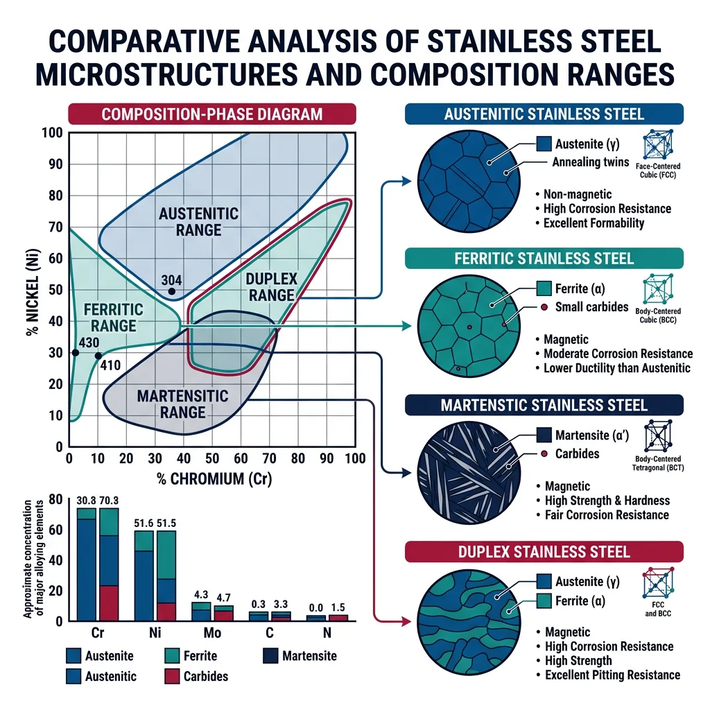
- Austenitic (300 series): FCC structure, non-magnetic, excellent corrosion resistance, highly formable. 304 (18Cr-8Ni, the "18/8" standard) for kitchen sinks and food equipment. 316 (16Cr-10Ni-2Mo) adds molybdenum for pitting resistance — used in marine and chemical environments. ~70% of all stainless steel produced.
- Ferritic (400 series): BCC structure, magnetic, lower cost (no Ni). 430 (16-18Cr) for automotive trim, appliances. Good oxidation resistance but less formable than austenitic.
- Martensitic (400 series): Heat-treatable for high hardness. 410 (12-14Cr) for turbine blades, cutlery, surgical instruments. 440C (16-18Cr, 0.95-1.2C) for premium knife blades and bearings.
- Duplex: Mixed austenite + ferrite (~50/50). Combines strength of ferritic with corrosion resistance of austenitic. 2205 (22Cr-5Ni-3Mo) for offshore oil platforms, desalination plants. Twice the yield strength of 316L.
Tool steels are special alloy steels designed for cutting, forming, and shaping other materials. Key families include:
- D2 (cold-work): 1.5% C, 12% Cr — air-hardening, excellent wear resistance. Used for punching dies, blanking tools
- M2 (high-speed): 0.85% C, 6% W, 5% Mo — retains hardness at red heat (~600°C). Used for drill bits, end mills, taps
- H13 (hot-work): 0.40% C, 5% Cr, 1.5% Mo, 1% V — resists thermal fatigue. Used for die-casting dies, extrusion tooling
HSLA (High-Strength Low-Alloy) steels contain small amounts of Nb, V, and Ti (each <0.1%) that form tiny carbide/nitride precipitates, dramatically increasing strength without sacrificing weldability. They're the unsung heroes behind lighter, more fuel-efficient vehicles and stronger pipelines.
import numpy as np
import matplotlib.pyplot as plt

# Compare compositions of common stainless steels
grades = ['304', '316', '430', '410', '2205 Duplex']
cr_content = [18, 16, 17, 13, 22]
ni_content = [8, 10, 0, 0, 5]
mo_content = [0, 2, 0, 0, 3]

x = np.arange(len(grades))
width = 0.25

fig, ax = plt.subplots(figsize=(10, 6))
bars1 = ax.bar(x - width, cr_content, width, label='Chromium (Cr)',
               color='#3B9797')
bars2 = ax.bar(x, ni_content, width, label='Nickel (Ni)',
               color='#BF092F')
bars3 = ax.bar(x + width, mo_content, width, label='Molybdenum (Mo)',
               color='#132440')

ax.set_xlabel('Stainless Steel Grade', fontsize=12, fontweight='bold')
ax.set_ylabel('Composition (wt%)', fontsize=12, fontweight='bold')
ax.set_title('Alloying Element Comparison in Stainless Steels',
             fontsize=14, fontweight='bold')
ax.set_xticks(x)
ax.set_xticklabels(grades, fontweight='bold')
ax.legend()
ax.grid(axis='y', alpha=0.3)

# Add value labels on bars
for bars in [bars1, bars2, bars3]:
    for bar in bars:
        height = bar.get_height()
        if height > 0:
            ax.annotate(f'{height}%', xy=(bar.get_x() + bar.get_width()/2, height),
                        xytext=(0, 3), textcoords="offset points",
                        ha='center', va='bottom', fontsize=9)

plt.tight_layout()
plt.show()
Stainless Steel in Medical Implants — 316L's Bio-Journey
316L stainless steel (the "L" means low carbon, ≤0.03% C) has been the workhorse of orthopedic implants for over 50 years — bone plates, screws, hip nails, and spinal rods. Its combination of corrosion resistance (from Cr and Mo), biocompatibility (low ion release), and mechanical strength makes it ideal for temporary fixation devices. The low carbon content prevents sensitization — a dangerous phenomenon where chromium carbides form at grain boundaries during welding, creating chromium-depleted zones vulnerable to intergranular corrosion. Inside the human body (pH ~7.4, 37°C, chloride-rich), this protection is critical. However, 316L has been gradually replaced by titanium alloys (Ti-6Al-4V) for permanent implants due to titanium's superior biocompatibility and lower elastic modulus (closer to bone's ~20 GPa vs steel's ~200 GPa), which reduces stress shielding — bone loss caused by an implant carrying too much load.
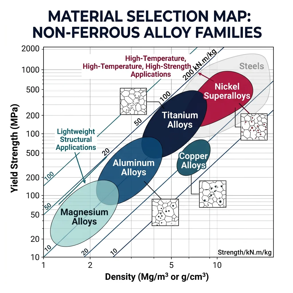
Non-Ferrous Alloys
While steel dominates by tonnage, non-ferrous metals — those without iron as the principal element — are essential wherever you need low density (aluminum, magnesium), high electrical conductivity (copper), corrosion immunity (titanium), or extreme temperature resistance (nickel superalloys). If steel is the reliable pickup truck, non-ferrous alloys are the Formula 1 cars — specialized, high-performance, and more expensive.
Aluminum alloys are classified by a four-digit system where the first digit identifies the principal alloying element:
- 1xxx (99%+ Al): Excellent corrosion resistance, high conductivity. Foil, electrical conductors, chemical equipment.
- 2xxx (Al-Cu): Heat-treatable, high strength. 2024-T3 for aircraft fuselage skins. Poor corrosion resistance — needs cladding.
- 3xxx (Al-Mn): Moderate strength, good formability. Beverage cans (3004), cooking utensils.
- 5xxx (Al-Mg): Good weldability, marine corrosion resistance. Boat hulls (5083), pressure vessels.
- 6xxx (Al-Mg-Si): Medium strength, excellent extrudability. Architectural profiles, bicycle frames (6061-T6).
- 7xxx (Al-Zn): Highest strength aluminum alloys. 7075-T6 for wing spars, landing gear components. Ultimate tensile strength ~570 MPa.
Temper designations tell you the processing history of the alloy: O = fully annealed (softest); H = strain-hardened (cold-worked); T4 = solution treated + naturally aged; T6 = solution treated + artificially aged (peak hardness); T73 = overaged for better stress-corrosion resistance (slightly lower strength than T6). The temper matters enormously — the same alloy 7075 has a yield strength of ~100 MPa in the O temper but ~500 MPa in the T6 temper.
import numpy as np
import matplotlib.pyplot as plt

# Density vs. Yield Strength for common aluminum alloys
alloys = ['1100-O', '3003-H14', '5052-H32', '6061-T6', '2024-T3', '7075-T6']
density = [2.71, 2.73, 2.68, 2.70, 2.78, 2.81]       # g/cm³
yield_str = [34, 145, 193, 276, 345, 503]              # MPa
uts = [90, 152, 228, 310, 483, 572]                    # MPa

fig, ax = plt.subplots(figsize=(10, 7))
scatter = ax.scatter(density, yield_str, s=200, c=yield_str,
                     cmap='RdYlGn', edgecolors='black', linewidth=1.5,
                     zorder=5)

# Label each point
for i, alloy in enumerate(alloys):
    ax.annotate(alloy, (density[i], yield_str[i]),
                textcoords="offset points", xytext=(12, 5),
                fontsize=10, fontweight='bold')

# Add arrows showing strength increase direction
ax.annotate('', xy=(2.81, 520), xytext=(2.70, 50),
            arrowprops=dict(arrowstyle='->', color='gray',
                            lw=2, ls='--'))
ax.text(2.74, 260, 'Increasing\nstrength →', fontsize=10,
        color='gray', rotation=70, ha='center')

ax.set_xlabel('Density (g/cm³)', fontsize=13, fontweight='bold')
ax.set_ylabel('Yield Strength (MPa)', fontsize=13, fontweight='bold')
ax.set_title('Aluminum Alloys: Density vs. Yield Strength',
             fontsize=14, fontweight='bold')
ax.grid(True, alpha=0.3)
plt.colorbar(scatter, label='Yield Strength (MPa)')
plt.tight_layout()
plt.show()
Boeing 787 and Aluminum-Lithium Alloys
While the Boeing 787 Dreamliner is famous for its 50% composite airframe, what's less known is that its remaining metallic structure uses third-generation aluminum-lithium (Al-Li) alloys like 2050-T84 and 2198-T8. Adding just 1–2% lithium to aluminum achieves two remarkable effects: (1) it reduces density by ~3% per 1% Li added (lithium is the lightest metallic element), and (2) it increases elastic modulus by ~6% per 1% Li added. The result is an alloy that is both lighter and stiffer than conventional 2024 or 7075. The Airbus A380 floor beams use Al-Li 2196, saving ~800 kg per aircraft. However, Al-Li alloys are more expensive, more anisotropic (properties vary with direction), and require careful processing to avoid delamination — trade-offs that keep engineers constantly balancing performance and cost.
Copper & Titanium Alloys
Copper alloys have served humanity for over 10,000 years — the "Copper Age" predates the Bronze Age. Copper's exceptional electrical conductivity (second only to silver) and thermal conductivity make it indispensable for wiring and heat exchangers. Its alloys offer a vast range of properties:
- Brass (Cu-Zn): Adding zinc increases strength and machinability while maintaining good corrosion resistance. C26000 (70Cu-30Zn) "cartridge brass" for ammunition casings. C36000 (61.5Cu-35.5Zn-3Pb) "free-cutting brass" for screw-machined parts — the most machinable common alloy.
- Bronze (Cu-Sn): Tin adds hardness and corrosion resistance. Phosphor bronze (C51000) for springs and electrical contacts. Aluminum bronze (C95400) for marine propellers — extraordinary seawater corrosion resistance.
- Cupronickel (Cu-Ni): 70Cu-30Ni for marine condensers, desalination plants, and — famously — coinage (U.S. nickels and many world coins).
- Beryllium copper (Cu-Be, ~2% Be): The only copper alloy that can be precipitation-hardened to very high strengths (~1200 MPa). Used for non-sparking tools in explosive atmospheres and high-reliability springs in aerospace connectors.
Titanium alloys combine an extraordinary set of properties: high strength, low density (4.51 g/cm³ — 60% of steel), excellent corrosion resistance, and biocompatibility. The "workhorse" alloy is Ti-6Al-4V (Grade 5), which accounts for over 50% of all titanium used commercially.
Titanium alloys are classified by their room-temperature microstructure:
- Alpha (α) alloys: HCP crystal structure, good creep resistance, weldable. Used at cryogenic temperatures (e.g., Ti-5Al-2.5Sn for liquid hydrogen tanks).
- Beta (β) alloys: BCC crystal structure, cold-formable, heat-treatable to very high strengths. Ti-15V-3Cr-3Al-3Sn for aircraft springs and fasteners.
- Alpha-Beta alloys: Mixed microstructure, optimized balance of properties. Ti-6Al-4V — 6% aluminum (α stabilizer) + 4% vanadium (β stabilizer). Used for jet engine compressor disks, orthopedic implants, and aerospace fasteners.
The SR-71 Blackbird's Titanium Skin
The SR-71 Blackbird, cruising at Mach 3.2 (3,530 km/h), experienced airframe temperatures exceeding 300°C due to aerodynamic heating — temperatures that would soften aluminum alloys. Lockheed's legendary Skunk Works, led by Kelly Johnson, made the radical decision to build 93% of the airframe from Ti-6Al-4V (Beta-120VCA) titanium. This was the 1960s, and titanium machining was in its infancy. The team discovered (often through costly failures) that titanium is sensitive to chlorine contamination — parts washed in Burbank's chlorinated tap water developed stress corrosion cracks. They switched to distilled water. Cadmium-plated tools left traces that caused embrittlement. Standard shop markers (containing chlorinated solvents) caused cracking. Every detail mattered. The program consumed so much titanium that the CIA had to set up fake companies to purchase it from the Soviet Union — the world's largest titanium producer — without revealing its military purpose.
Superalloys & Refractory Metals
Superalloys are the elite materials of extreme-temperature engineering. Designed to maintain structural integrity above 540°C — where most steels and aluminum alloys would fail — they enable the hottest sections of jet engines and gas turbines. The name "superalloy" comes from their superhuman temperature capability, not from having superpowers (though they come close).
- Nickel-based (~50% of superalloys): The most critical. FCC γ matrix strengthened by ordered γ' (Ni₃(Al,Ti)) precipitates. Inconel 718 (53Ni-19Cr-18Fe-5Nb) for turbine disks. Waspaloy (58Ni-19Cr-13Co-4Mo-3Ti-1.4Al) for turbine cases. CMSX-4 (single crystal) for the hottest turbine blades, operating at ~1050°C — about 80% of their melting point.
- Cobalt-based: Better hot corrosion resistance than Ni-based. Stellite 6 (Co-28Cr-4W-1C) for wear-resistant valve seats, saw tips. Haynes 188 (Co-22Cr-22Ni-14W) for combustor liners.
- Iron-based superalloys: Lower cost, lower temperature capability. A-286 (Fe-25Ni-15Cr-2Ti-1.5Mo) for automotive turbocharger wheels, exhaust valves. Useful up to ~700°C.
Refractory metals push even beyond superalloys into the >2000°C regime:
- Tungsten (W): Melting point 3422°C — highest of all metals. Used for light bulb filaments, rocket nozzle throats, armor-piercing projectiles. Density: 19.3 g/cm³ (heavier than gold).
- Molybdenum (Mo): Melting point 2623°C. Used for furnace heating elements, TZM alloy (Mo-0.5Ti-0.1Zr) for rocket engine components. Better oxidation resistance than W.
- Tantalum (Ta): Exceptional corrosion resistance — immune to most acids. Used for surgical implants, capacitors in electronics, and chemical reactor linings.
- Rhenium (Re): Melting point 3186°C. Added to nickel superalloys (3-6%) to improve creep resistance. Extremely rare and expensive (~$3,000/kg).
The evolution of turbine blade technology represents materials engineering at its finest: early blades were equiaxed polycrystals (many small, randomly oriented grains). Creep failure originated at grain boundaries perpendicular to the blade's centrifugal load. The solution? Directional solidification (DS) — controlling cooling to produce columnar grains aligned with the stress axis, eliminating transverse grain boundaries. The ultimate step was single-crystal (SX) blades — no grain boundaries at all — increasing temperature capability by another 25–50°C. Modern SX blades (like CMSX-10) contain up to 10 alloying elements and operate at temperatures above their bulk melting point, surviving only because of sophisticated internal cooling channels and thermal barrier coatings (TBCs).
GE90 Turbine Blades: Engineering at 1,500°C
The GE90-115B engine (powering the Boeing 777) produces 115,000 lbs of thrust — the most powerful jet engine ever certified. Its high-pressure turbine blades experience combustion gas temperatures of ~1,500°C while rotating at 9,332 RPM, each blade experiencing centrifugal forces equivalent to hanging a fully loaded double-decker bus from it. The blades are single-crystal René N5 superalloy, investment-cast with intricate internal cooling channels just 0.5 mm wide, through which compressor bleed air flows. A thermal barrier coating (TBC) of yttria-stabilized zirconia (YSZ, ~0.25 mm thick) provides a thermal drop of ~170°C at the blade surface. Without cooling and TBC, the blades would melt. Each blade costs approximately $10,000 and is inspected by CT scan for internal channel integrity before installation. The turbine entry temperature of modern military engines (like the F135 in the F-35) pushes even higher — approaching the theoretical limits of nickel-based superalloys and driving research into ceramic matrix composites (CMCs).
Strengthening Mechanisms
Here's a fundamental question that drives all of physical metallurgy: Why are pure metals so much softer than we'd expect from their atomic bonds? The theoretical strength of a perfect crystal — calculated from the force needed to simultaneously break a plane of atomic bonds — is roughly $E/10$ (one-tenth of the elastic modulus). For iron, this predicts a strength of ~21 GPa. But actual pure iron yields at a mere ~50 MPa — over 400 times lower than theory.
The Cookie Dough Analogy: Imagine pressing on a ball of cookie dough. It deforms easily because the dough can flow — molecules slide past each other. If you add chocolate chips, chocolate chunks, and nuts, the dough gets stiffer because these inclusions block the flow of dough around them. Metals work the same way: atoms deform by the motion of dislocations (line defects in the crystal lattice), and every strengthening mechanism works by making dislocation motion more difficult — like adding obstacles to the cookie dough.
graph TD
    SM["Strengthening
Mechanisms"]

    SS["Solid Solution
Strengthening"]
    GB["Grain Boundary
Strengthening
(Hall-Petch)"]
    PH["Precipitation
Hardening
(Age Hardening)"]
    WH["Work Hardening
(Cold Working /
Strain Hardening)"]

    SM --> SS
    SM --> GB
    SM --> PH
    SM --> WH

    SS --> SSE["Solute atoms distort
lattice, impede
dislocation motion"]
    GB --> GBE["Grain boundaries
block slip planes;
smaller grains = stronger"]
    PH --> PHE["Fine precipitates
pin dislocations
(Orowan mechanism)"]
    WH --> WHE["Increased dislocation
density creates
tangles and barriers"]

    style SM fill:#132440,stroke:#132440,color:#fff
    style SS fill:#e8f4f4,stroke:#3B9797
    style GB fill:#f0f4f8,stroke:#16476A
    style PH fill:#fff5f5,stroke:#BF092F
    style WH fill:#e8f4f4,stroke:#3B9797
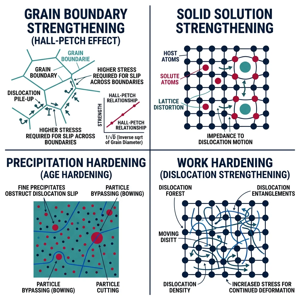
- 1. Grain Boundary Strengthening (Hall-Petch) — Smaller grains = more grain boundaries = more obstacles to dislocation motion
- 2. Solid Solution Strengthening — Foreign atoms distort the lattice and create stress fields that hinder dislocations
- 3. Precipitation/Dispersion Hardening — Tiny second-phase particles force dislocations to cut through or bow around them
- 4. Work Hardening (Strain Hardening) — Deforming the metal creates more dislocations that tangle and block each other
Grain Boundary Strengthening: The Hall-Petch Relation
When a dislocation traveling through one grain reaches a grain boundary, it cannot easily cross into the neighboring grain because the adjacent grain has a different crystallographic orientation. The dislocation "piles up" at the boundary, and a new dislocation must be nucleated in the next grain — which requires additional stress. The more grain boundaries (i.e., the smaller the grains), the more frequently this blocking occurs.
This relationship is captured by the Hall-Petch equation:
$\sigma_y = \sigma_0 + k_y \cdot d^{-1/2}$
Where $\sigma_y$ is the yield strength, $\sigma_0$ is the friction stress (lattice resistance to dislocation motion), $k_y$ is the Hall-Petch slope (a material constant), and $d$ is the average grain diameter.
Solid Solution Strengthening
Adding foreign atoms into the host lattice creates local strain fields that interact with dislocations. There are two types:
- Substitutional: The solute atom replaces a host atom (similar size). Example: zinc (Zn) in copper (Cu) → brass. The size difference between Cu (128 pm) and Zn (134 pm) creates lattice strain.
- Interstitial: Small solute atoms fit between host atoms. Example: carbon (77 pm) in iron's BCC lattice. Carbon is small enough to occupy octahedral interstitial sites, creating a much larger strain field than substitutional atoms — which is why even tiny amounts of carbon strengthen iron dramatically.
import numpy as np
import matplotlib.pyplot as plt

# Hall-Petch demonstration for mild steel
# sigma_y = sigma_0 + k_y * d^(-1/2)
sigma_0 = 70     # MPa, friction stress for low carbon steel
k_y = 0.74       # MPa·m^(1/2), Hall-Petch coefficient for steel

# Grain diameters from 1 mm down to 100 nm (0.0001 mm)
d_mm = np.logspace(-1, 3, 200)  # in micrometers
d_m = d_mm * 1e-6               # convert to meters

sigma_y = sigma_0 + k_y * d_m**(-0.5)  # Hall-Petch

fig, ax = plt.subplots(figsize=(10, 6))
ax.plot(d_mm, sigma_y, 'b-', linewidth=2.5, label='Hall-Petch prediction')

# Mark specific grain sizes
grain_examples = {
    'Coarse (100 μm)': 100,
    'Fine (10 μm)': 10,
    'Ultrafine (1 μm)': 1,
    'Nanocrystalline (0.1 μm)': 0.1,
}

for label, d_val in grain_examples.items():
    d_val_m = d_val * 1e-6
    sy = sigma_0 + k_y * d_val_m**(-0.5)
    ax.plot(d_val, sy, 'ro', markersize=10, zorder=5)
    ax.annotate(f'{label}\nσ_y = {sy:.0f} MPa',
                xy=(d_val, sy), textcoords="offset points",
                xytext=(15, 15), fontsize=9,
                arrowprops=dict(arrowstyle='->', color='red'))

ax.set_xscale('log')
ax.set_xlabel('Grain Diameter (μm)', fontsize=13, fontweight='bold')
ax.set_ylabel('Yield Strength (MPa)', fontsize=13, fontweight='bold')
ax.set_title('Hall-Petch Relationship: Grain Size vs. Strength (Steel)',
             fontsize=14, fontweight='bold')
ax.legend(fontsize=11)
ax.grid(True, alpha=0.3, which='both')
ax.invert_xaxis()
plt.tight_layout()
plt.show()

print("Key insight: Reducing grain size from 100 μm to 1 μm")
d1, d2 = 100e-6, 1e-6
s1 = sigma_0 + k_y * d1**(-0.5)
s2 = sigma_0 + k_y * d2**(-0.5)
print(f"increases yield strength from {s1:.0f} to {s2:.0f} MPa")
print(f"That's a {(s2-s1)/s1*100:.0f}% improvement!")
Nanocrystalline Metals — When Hall-Petch Breaks Down
The Hall-Petch equation predicts that strength increases without limit as grains get smaller. But experiments in the 1990s revealed a startling phenomenon: below grain sizes of roughly 10–20 nm, further refinement actually decreases strength — a phenomenon called the inverse Hall-Petch effect. At the nanoscale, a significant fraction of atoms sit at grain boundaries rather than in crystal interiors. Deformation shifts from dislocation-based plasticity (which grain boundaries impede) to grain boundary sliding and Coble creep (which grain boundaries facilitate). Think of it this way: if each grain is only 50 atoms across, there's no room for dislocations to form, and the material behaves more like a collection of loosely connected nanoparticles. This limit defines the frontier of grain refinement research and has practical implications for nanostructured coatings, thin films, and MEMS devices.
Precipitation Hardening
Precipitation hardening (also called age hardening) is the most potent strengthening mechanism for many aluminum, nickel, and titanium alloys. It can increase strength by 3–5 times over the annealed condition. The process works by creating a fine dispersion of nanometer-scale precipitate particles that block dislocation motion — like scattering thousands of tiny obstacles across a race track.
The Chocolate Chip Cookie Analogy: Imagine making cookies. In the "solutionize" step, you melt the chocolate chips into the dough at high temperature so they're fully dissolved (a uniform solution). Then you "quench" by rapidly chilling the dough in the fridge — the chocolate doesn't have time to separate out, so it's trapped in the dough as a supersaturated solution. Finally, you "age" at a moderate temperature — the chocolate slowly re-precipitates as tiny chips distributed uniformly throughout the dough, making it much harder to deform. That's precipitation hardening in a nutshell.
The three steps of precipitation hardening:
- Solution Treatment (Solutionize): Heat to a high temperature (e.g., 495°C for Al-Cu) to dissolve all solute atoms into a single-phase solid solution, just as sugar dissolves in hot water.
- Quench: Rapidly cool (usually in water) to trap the solute in a supersaturated solid solution — a metastable state where the lattice contains more solute than it wants.
- Age (Precipitate): Hold at an intermediate temperature (e.g., 190°C for hours) to allow the supersaturated solute to slowly cluster and form coherent precipitate particles. These particles create strain fields that impede dislocations.
In the classic Al-Cu system, the precipitation sequence during aging is:
SSSS → GP zones → θ'' → θ' → θ (Al₂Cu)
GP zones (Guinier-Preston zones) are Cu-rich planar clusters just 1–2 atoms thick. They're coherent with the aluminum matrix (matching lattice spacing), creating maximum strain and maximum hardening. As aging continues, these grow into θ'' and θ' precipitates — still semi-coherent and effective. Over-aging produces θ (Al₂Cu) — a coarse, incoherent equilibrium phase that has lost its coherency strain. The dislocations can now simply bypass these large particles rather than being blocked, so hardness decreases. This is why precise control of aging time and temperature is critical.
import numpy as np
import matplotlib.pyplot as plt

# Simulate aging curves for Al-Cu at different temperatures
time_hours = np.linspace(0, 100, 500)

def aging_curve(t, peak_hardness, time_to_peak, rate_decay):
    """Model: rise to peak then gradual decline (over-aging)."""
    rise = peak_hardness * (1 - np.exp(-3 * t / time_to_peak))
    decay = 1 - rate_decay * np.maximum(t - time_to_peak, 0) / time_to_peak
    decay = np.maximum(decay, 0.5)  # floor at 50% of peak
    return rise * decay

fig, ax = plt.subplots(figsize=(10, 6))

# Three aging temperatures
configs = [
    ('130°C (Low T)', 150, 60, 0.15, '#3B9797'),
    ('190°C (Optimal)', 180, 12, 0.25, '#BF092F'),
    ('230°C (High T)', 140, 3, 0.40, '#132440'),
]

for label, peak, t_peak, rate, color in configs:
    hardness = aging_curve(time_hours, peak, t_peak, rate)
    ax.plot(time_hours, hardness, linewidth=2.5, label=label, color=color)

# Mark key regions
ax.axvspan(0, 2, alpha=0.1, color='blue', label='GP zones forming')
ax.axvspan(8, 15, alpha=0.1, color='green', label='θ\'\'/θ\' (peak)')
ax.axvspan(40, 100, alpha=0.1, color='red', label='Over-aging (θ)')

# Labels
ax.annotate('PEAK\nHARDNESS', xy=(12, 178), fontsize=11,
            fontweight='bold', ha='center', color='#BF092F')
ax.annotate('OVER-AGED\n(coarse θ)', xy=(70, 115), fontsize=10,
            ha='center', color='red')

ax.set_xlabel('Aging Time (hours)', fontsize=13, fontweight='bold')
ax.set_ylabel('Hardness (HV)', fontsize=13, fontweight='bold')
ax.set_title('Precipitation Hardening Aging Curves — Al-Cu Alloy',
             fontsize=14, fontweight='bold')
ax.legend(loc='upper right', fontsize=9)
ax.set_ylim(0, 200)
ax.grid(True, alpha=0.3)
plt.tight_layout()
plt.show()

print("Optimal aging: 190°C for ~12 hours → peak hardness ~180 HV")
print("Under-aging: insufficient time → GP zones only → lower strength")
print("Over-aging: too long → coarse θ particles → strength drops")
Al 2024-T3 in Aircraft Fuselage Panels
2024-T3 (Al-4.4Cu-1.5Mg-0.6Mn) has been the standard fuselage skin material for commercial aircraft for over 60 years. The "T3" temper means it's solution-treated, cold-worked, and naturally aged at room temperature — a process that takes about 4 days to reach stable properties. Natural aging produces extremely fine GP zones that give 2024-T3 its excellent fatigue crack growth resistance — the most critical property for a pressurized fuselage that experiences ~60,000 pressure cycles over its service life (each takeoff and landing is one cycle). The Boeing 737 fuselage uses 2024-T3 sheets clad with pure aluminum (Alclad) on both sides — the pure aluminum layer sacrificially corrodes to protect the high-strength core, similar to how zinc galvanizing protects steel. This "Alclad 2024-T3" combination optimizes both fatigue resistance and corrosion performance simultaneously.
Heat Treatment Processes
Heat treatment is the metallurgist's primary tool for controlling microstructure and properties. By manipulating temperature and cooling rate, we can transform the same piece of steel from soft and ductile to hard and spring-like — without changing its chemical composition at all.
- Full Annealing: Heat above A3 line, slow furnace cool. Produces coarse pearlite — maximum softness and ductility. Used to make steel easy to machine or form.
- Normalizing: Heat above A3, air cool. Produces fine pearlite — slightly harder than annealed. The "default" condition for structural steels. Refines grain size and homogenizes composition.
- Stress Relief Annealing: Heat to 550–650°C (below A1), slow cool. Removes residual stresses from welding, casting, or machining without significantly changing microstructure.
- Quenching: Heat above A3, rapid cool in water/oil/polymer. If fast enough, austenite transforms to martensite — a supersaturated, distorted BCT structure that is extremely hard but brittle.
- Tempering: Reheat quenched martensite to 150–650°C. Carbon atoms diffuse to form tiny carbide particles, relieving internal stresses. Trading some hardness for greatly improved toughness. The higher the tempering temperature, the softer and tougher the result.
flowchart TD
    START["Raw Steel"] --> HEAT["Austenitize\n(Heat above Ac3)"]
    HEAT --> QUENCH{"Quench\nMedium?"}
    QUENCH -->|"Water"| WATER["Fast Cool\n→ Martensite"]
    QUENCH -->|"Oil"| OIL["Medium Cool\n→ Bainite + Martensite"]
    QUENCH -->|"Air"| AIR["Slow Cool\n→ Pearlite"]
    WATER --> TEMPER["Temper\n(Reheat 150-650°C)"]
    OIL --> TEMPER
    TEMPER --> FINAL["Final Properties\n(Hardness vs Toughness)"]
    AIR --> NORM["Normalized\nSteel"]
Quenching media differ in their cooling severity: water (fastest, can cause cracking from thermal shock) → 10% NaOH brine (even faster, used for maximum hardness) → polymer quenchant (PAG) (adjustable severity, fewer residual stresses) → oil (moderate, common for alloy steels) → air (slowest, for air-hardening steels like A2 and D2). The challenge is cooling fast enough to avoid pearlite/bainite formation while not so fast that thermal gradients cause distortion or quench cracking.
TTT (Time-Temperature-Transformation) diagrams show which phases form when you hold austenite at a constant temperature below A1. CCT (Continuous Cooling Transformation) diagrams show what happens during continuous cooling — closer to industrial practice. Both are essentially "maps" that tell you: "If you cool at this rate, you'll get this microstructure." Fast cooling paths veer left on the diagram, hitting the martensite start temperature (Ms) without intersecting the pearlite or bainite "noses."
Surface hardening techniques modify only the outer layer while keeping the core tough:
- Carburizing: Diffuse carbon into the surface at ~925°C in a carbon-rich atmosphere. Creates a high-carbon case (0.6–0.8 mm deep) on a low-carbon core. Then quench to form hard martensite at the surface. Used for gears and bearings.
- Nitriding: Diffuse nitrogen at ~525°C in an ammonia atmosphere. Nitrogen forms very hard nitrides (Fe₄N) at the surface without requiring a subsequent quench — minimal distortion. Used for crankshafts, precision parts.
import numpy as np
import matplotlib.pyplot as plt

# Simulate cooling curves for different quench media
time_sec = np.linspace(0, 120, 500)  # 0 to 120 seconds
T_initial = 850  # °C (austenitizing temperature)
T_ambient = 25

def cooling_curve(t, h_coeff, T0=T_initial, T_env=T_ambient):
    """Newton's law of cooling: T(t) = T_env + (T0 - T_env) * exp(-h*t)."""
    return T_env + (T0 - T_env) * np.exp(-h_coeff * t)

fig, ax = plt.subplots(figsize=(10, 7))

# Different quench media (approximate heat transfer coefficients)
media = [
    ('Still Air', 0.008, '#3B9797', '-'),
    ('Oil Quench', 0.035, '#16476A', '--'),
    ('Polymer (PAG)', 0.055, '#132440', '-.'),
    ('Water Quench', 0.12, '#BF092F', '-'),
    ('Brine (10% NaCl)', 0.18, '#8B0000', ':'),
]

for label, h, color, ls in media:
    T = cooling_curve(time_sec, h)
    ax.plot(time_sec, T, linewidth=2.5, label=label, color=color,
            linestyle=ls)

# Mark critical temperatures
ax.axhline(y=727, color='purple', linestyle='--', alpha=0.5, linewidth=1)
ax.text(115, 735, 'A1 (727°C)', fontsize=9, color='purple')
ax.axhline(y=230, color='orange', linestyle='--', alpha=0.5, linewidth=1)
ax.text(115, 238, 'Ms (~230°C)', fontsize=9, color='orange')

# Shade martensite formation zone
ax.axhspan(100, 230, alpha=0.08, color='red')
ax.text(60, 160, 'Martensite\nformation zone', fontsize=10,
        ha='center', color='#BF092F', fontweight='bold')

ax.set_xlabel('Time (seconds)', fontsize=13, fontweight='bold')
ax.set_ylabel('Temperature (°C)', fontsize=13, fontweight='bold')
ax.set_title('Cooling Curves for Different Quenching Media (1045 Steel)',
             fontsize=14, fontweight='bold')
ax.legend(loc='upper right', fontsize=10)
ax.set_ylim(0, 900)
ax.grid(True, alpha=0.3)
plt.tight_layout()
plt.show()

print("Key: To form martensite, the cooling curve must pass through")
print("727°C → 230°C fast enough to avoid the pearlite/bainite 'nose'")
print("on the CCT diagram (typically < 1-5 seconds for plain carbon steel).")
Degradation & Frontier Alloys
Metals don't just sit there and stay strong forever. At elevated temperatures, metals progressively weaken as thermal energy helps atoms move, vacancies diffuse, and dislocations climb over obstacles they'd be blocked by at room temperature. As a rough rule of thumb, significant thermally-activated degradation begins above approximately 0.3–0.4 Tm (melting temperature in Kelvin).
Creep is the slow, continuous deformation of a material under a constant stress at elevated temperature — even stresses well below the room-temperature yield strength can cause failure given enough time. Think of it like a glacier: ice is rigid at everyday timescales, but over years it flows slowly under its own weight. Metals behave similarly when hot enough.
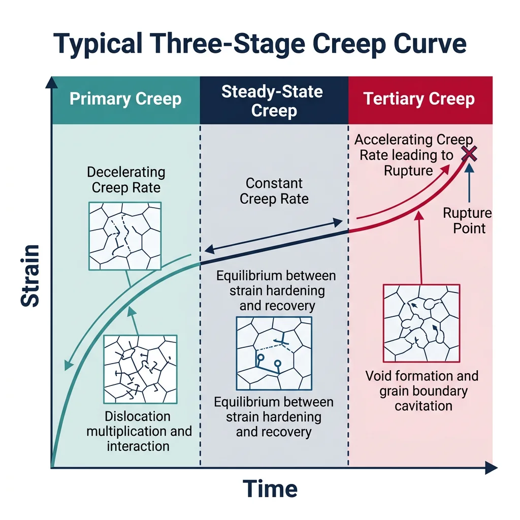
- Primary (Transient) Creep: Strain rate decreases with time. Dislocations encounter barriers and pile up. Work hardening dominates. The material is "digging in" against further deformation.
- Secondary (Steady-State) Creep: Strain rate becomes constant — a balance between work hardening and thermally-assisted recovery. This stage dominates the creep life and is used for design calculations. The steady-state creep rate $\dot{\epsilon}$ follows the Arrhenius relationship: $\dot{\epsilon} = A \sigma^n \exp(-Q/RT)$, where $Q$ is the activation energy, $n$ is the stress exponent (typically 3–8), and $T$ is absolute temperature.
- Tertiary Creep: Strain rate accelerates rapidly. Grain boundary voids nucleate and link up (cavitation), internal necking occurs, and the cross-section reduces until catastrophic fracture. This is the "death spiral" of creep.
Creep mechanisms depend on the stress and temperature regime:
- Dislocation creep (power-law creep): At high stresses, dislocations climb over obstacles by absorbing/emitting vacancies. Dominates in typical engineering applications. Stress exponent $n$ ≈ 3–8.
- Nabarro-Herring creep: At very high temperatures and low stresses, vacancies diffuse through the grain interior (lattice diffusion). $n$ ≈ 1 (linear in stress). Strain rate inversely proportional to $d^2$ (grain size squared).
- Coble creep: Vacancies diffuse along grain boundaries (faster paths) instead of through the lattice. Dominant for fine-grained materials at moderate temperatures. $n$ ≈ 1, inversely proportional to $d^3$.
The Larson-Miller parameter (LMP) is a powerful engineering tool that collapses creep data at different temperatures and times onto a single master curve: $\text{LMP} = T(C + \log t_r)$, where $T$ is temperature in Kelvin, $t_r$ is rupture time in hours, and $C$ is a material constant (typically ~20 for steels). By plotting stress versus LMP, engineers can predict creep life at one temperature based on shorter tests at higher temperatures — an essential technique since real-world creep lives can span 30+ years.
import numpy as np
import matplotlib.pyplot as plt

# Simulate a classic three-stage creep curve
total_time = 1000  # hours
t = np.linspace(0.1, total_time, 2000)

def creep_curve(t, eps_0=0.002, A_primary=0.008, n_primary=0.33,
                rate_ss=2e-5, t_tertiary=800, B_tert=1e-8):
    """Three-stage creep: primary + steady-state + tertiary."""
    # Primary: decelerating (power law)
    primary = A_primary * t**n_primary
    # Steady-state: linear
    steady = rate_ss * t
    # Tertiary: accelerating (exponential after onset)
    tertiary = np.where(t > t_tertiary,
                        B_tert * (t - t_tertiary)**3, 0)
    return eps_0 + primary + steady + tertiary

strain = creep_curve(t)

fig, (ax1, ax2) = plt.subplots(1, 2, figsize=(14, 6))

# Left: Creep curve (strain vs time)
ax1.plot(t, strain * 100, 'b-', linewidth=2.5)
ax1.axvspan(0, 100, alpha=0.1, color='green')
ax1.axvspan(100, 800, alpha=0.1, color='blue')
ax1.axvspan(800, 1000, alpha=0.15, color='red')
ax1.text(50, 0.6, 'I\nPrimary', ha='center', fontweight='bold',
         color='green', fontsize=11)
ax1.text(450, 0.6, 'II\nSteady-State', ha='center', fontweight='bold',
         color='blue', fontsize=11)
ax1.text(900, 0.6, 'III\nTertiary', ha='center', fontweight='bold',
         color='red', fontsize=11)
ax1.set_xlabel('Time (hours)', fontsize=13, fontweight='bold')
ax1.set_ylabel('Creep Strain (%)', fontsize=13, fontweight='bold')
ax1.set_title('Three Stages of Creep', fontsize=14, fontweight='bold')
ax1.grid(True, alpha=0.3)

# Right: Creep rate vs time
dt = np.diff(t)
d_strain = np.diff(strain)
creep_rate = d_strain / dt
t_mid = (t[:-1] + t[1:]) / 2

ax2.semilogy(t_mid, creep_rate, 'r-', linewidth=2)
ax2.set_xlabel('Time (hours)', fontsize=13, fontweight='bold')
ax2.set_ylabel('Creep Rate (1/hr)', fontsize=13, fontweight='bold')
ax2.set_title('Creep Rate vs. Time', fontsize=14, fontweight='bold')
ax2.axvline(x=100, color='gray', linestyle='--', alpha=0.5)
ax2.axvline(x=800, color='gray', linestyle='--', alpha=0.5)
ax2.text(450, creep_rate[len(creep_rate)//2], 'Minimum\ncreep rate',
         ha='center', fontsize=10, fontweight='bold', color='blue')
ax2.grid(True, alpha=0.3)

plt.tight_layout()
plt.show()

print("Design principle: Components are designed based on the")
print("steady-state (minimum) creep rate — typically allowing")
print("no more than 1% total creep strain over the design life.")
Jet Engine Turbine Blade Creep Life Prediction
A first-stage turbine blade in a commercial aero-engine operates at roughly 1050°C under a centrifugal stress of ~140 MPa for a required service life of 20,000 hours (~7 years of operation). Using the Larson-Miller approach, engineers conduct accelerated creep tests: they test at 1100°C and 140 MPa, where rupture occurs in 500 hours, and at 1150°C where rupture occurs in just 50 hours. Plotting both on LMP vs. stress coordinates, they fall on the same master curve, confirming the material model. Extrapolating to 1050°C predicts a rupture life of ~35,000 hours — providing a safety factor of 1.75× on the 20,000-hour requirement. However, the blade also experiences thermal cycling (engine start/stop), hot corrosion from ingested salt, and foreign object damage — all of which reduce the actual life below the ideal creep prediction. This is why certification requires both analytical prediction and extensive rig testing.
Fatigue & Cyclic Loading
Fatigue is the progressive, localized structural damage that occurs when a material is subjected to cyclic (repetitive) loading — even when the maximum stress in each cycle is well below the material's static yield strength. It's the most common cause of mechanical failure in engineering components — responsible for an estimated 80–90% of all structural failures.
The Paper Clip Analogy: Take a paper clip and bend it back and forth. It doesn't break on the first bend — or the fifth. But after perhaps 10–20 cycles, it snaps. Yet the stress you applied each time was far below what it would take to pull the clip apart in tension. That's fatigue in action: each cycle creates a tiny amount of damage (microscopic crack growth), and these damages accumulate until the remaining cross-section can no longer sustain the load.
The fatigue process has three stages:
- Crack Initiation: Microcracks form at stress concentrations — surface scratches, inclusions, grain boundaries, or sharp geometric features. This can consume most of the fatigue life (>90%) in smooth, polished specimens.
- Crack Propagation: Once a crack reaches a critical size (typically a few grain diameters), it enters Stage II growth — advancing with each loading cycle by a small increment. The growth rate follows the Paris law: $da/dN = C(\Delta K)^m$, where $da/dN$ is crack growth per cycle, $\Delta K$ is the stress intensity factor range, and $C$ and $m$ are material constants.
- Final Fracture: When the crack has grown so large that the remaining cross-section cannot sustain the peak load, catastrophic fracture occurs — typically suddenly and without warning.
S-N curves (stress vs. number of cycles to failure, aka Wöhler curves) characterize a material's fatigue behavior. For ferrous metals (steel, iron), there's typically an endurance limit — a stress below which the material can theoretically endure infinite cycles (typically ~0.4–0.5 of UTS for wrought steels). Aluminum alloys, unfortunately, have no true endurance limit — they will eventually fail at any stress level, which is why aircraft must be inspected and retired after a specified number of cycles.
Miner's rule provides a simple estimate for cumulative fatigue damage under variable-amplitude loading: $\sum (n_i / N_{f,i}) = 1$ at failure, where $n_i$ is the number of cycles at stress level $i$ and $N_{f,i}$ is the fatigue life at that stress. While not perfectly accurate, it's widely used for preliminary design.
Three fatigue design philosophies:
- Safe-life: Design so the component never cracks during its planned service life, then retire it. Used for helicopter rotor hubs, landing gear.
- Damage-tolerant: Assume cracks will form. Design so they grow slowly enough to be detected during scheduled inspections before reaching critical size. Used for airplane fuselages.
- Fail-safe: Design redundant load paths so that if one element fails, others carry the load. Used for wing structures with multiple spars.
import numpy as np
import matplotlib.pyplot as plt

# S-N (Wöhler) curves for steel vs. aluminum alloy
cycles = np.logspace(3, 9, 500)  # 10^3 to 10^9 cycles

# Steel (with endurance limit at ~240 MPa)
def sn_steel(N, Su=500, Se=240, N_transition=1e6):
    b = -np.log10(Su / Se) / np.log10(N_transition / 1e3)
    a = Su / (1e3 ** b)
    S = a * N ** b
    S = np.maximum(S, Se)  # endurance limit floor
    return S

# Aluminum (no true endurance limit)
def sn_aluminum(N, Su=350, S_ref=120, b=-0.09):
    S = Su * (N / 1e3) ** b
    return S

fig, ax = plt.subplots(figsize=(10, 7))

stress_steel = sn_steel(cycles)
stress_al = sn_aluminum(cycles)

ax.semilogx(cycles, stress_steel, 'b-', linewidth=2.5,
            label='Medium Carbon Steel (AISI 1045)')
ax.semilogx(cycles, stress_al, 'r--', linewidth=2.5,
            label='Aluminum 6061-T6')

# Mark endurance limit for steel
ax.axhline(y=240, color='blue', linestyle=':', alpha=0.4)
ax.text(1e8, 248, 'Steel Endurance Limit (~240 MPa)',
        fontsize=9, color='blue')

# Mark 10^7 fatigue limit for aluminum
al_at_1e7 = sn_aluminum(1e7)
ax.plot(1e7, al_at_1e7, 'ro', markersize=8)
ax.annotate(f'Al "fatigue limit"\nat 10⁷ cycles: {al_at_1e7:.0f} MPa',
            xy=(1e7, al_at_1e7), textcoords="offset points",
            xytext=(15, 15), fontsize=9,
            arrowprops=dict(arrowstyle='->', color='red'))

ax.set_xlabel('Number of Cycles to Failure (N)', fontsize=13,
              fontweight='bold')
ax.set_ylabel('Stress Amplitude (MPa)', fontsize=13, fontweight='bold')
ax.set_title('S-N Curves: Steel vs. Aluminum', fontsize=14,
             fontweight='bold')
ax.legend(fontsize=11)
ax.grid(True, alpha=0.3, which='both')
ax.set_ylim(50, 550)
plt.tight_layout()
plt.show()

print("Key difference: Steel has a true endurance limit (~240 MPa)")
print("below which it can endure infinite cycles.")
print("Aluminum has NO endurance limit — it will eventually fail")
print("at any stress level, hence mandatory retirement lives in aviation.")
The De Havilland Comet Disasters — Fatigue in Aviation History
In 1954, two De Havilland Comet jetliners — the world's first commercial jet aircraft — disintegrated in flight over the Mediterranean within months of each other, killing all aboard. The investigation, led by the Royal Aircraft Establishment at Farnborough, was one of the most thorough failure analyses in engineering history. By pressurizing a salvaged fuselage in a water tank and cycling it to simulate flights, investigators discovered that fatigue cracks originated at the square-cornered windows — specifically at the corner rivet holes of the ADF (automatic direction finder) window. The square corners acted as severe stress concentrators, amplifying the cyclic hoop stress from cabin pressurization by a factor of ~3×. After only ~1,300 pressurization cycles, the cracks reached critical length and the fuselage failed explosively in a fraction of a second. The disaster transformed aviation engineering: all future aircraft adopted rounded windows (stress concentration factor reduced from ~3 to ~1.5), fail-safe design (crack stoppers, redundant structure), and mandatory fatigue testing. The Comet's sacrifice wrote the rulebook that keeps every modern airliner flying safely.
High-Entropy & Lightweight Alloys
For over 5,000 years, alloy design followed a simple recipe: pick one principal element (iron, aluminum, copper, nickel) and add small amounts of others to modify properties. Steel is iron with a dash of carbon. Bronze is copper with a splash of tin. This paradigm works — but it explores only a tiny fraction of the vast composition space available.
High-Entropy Alloys (HEAs) shatter this paradigm. Instead of one dominant element, they contain five or more principal elements in roughly equal proportions (each 5–35 at%). The result is an alloy sitting at the center of a multi-component phase diagram — a region that traditional metallurgy never explored because conventional wisdom assumed it would produce a chaotic mess of intermetallic phases. Instead, the high configurational entropy ($\Delta S_{mix} = -R \sum x_i \ln x_i$) of mixing often stabilizes simple solid-solution phases — typically FCC, BCC, or a combination.
- 1. High-Entropy Effect: The large mixing entropy (ΔSmix ≥ 1.5R for 5+ elements) stabilizes simple solid solutions over ordered intermetallics, especially at high temperatures where TΔS dominates the Gibbs free energy.
- 2. Sluggish Diffusion: Each atom is surrounded by different neighbors, creating a rugged energy landscape for diffusion. Atoms move slowly, enhancing creep resistance and phase stability at high temperatures.
- 3. Severe Lattice Distortion: Different-sized atoms sharing the same lattice create massive internal strain fields — acting as "distributed solid solution strengthening" throughout the entire crystal, not just around isolated solute atoms.
- 4. Cocktail Effect: Properties can exceed the rule-of-mixtures average — synergistic interactions between elements produce unexpected improvements. Like a cocktail that tastes better than any individual ingredient.
The Cantor alloy (CrMnFeCoNi), discovered by Brian Cantor in 2004, forms a single FCC solid solution and displays remarkable properties: exceptional fracture toughness at cryogenic temperatures (>200 MPa·√m at 77K — rivaling the best engineering alloys), good strength, and outstanding ductility. It defies the usual strength-ductility trade-off that plagues conventional alloys.
Lightweight HEAs for automotive and aerospace use low-density elements: AlTiVCrNb and AlCrFeMnNi-type systems targeting densities of 5–6 g/cm³ (between aluminum and titanium) with superior high-temperature strength. These are still in the research phase but hold enormous promise.
Metallic glasses (amorphous metals) represent another frontier — metals cooled so rapidly (>10⁶ K/s for most alloys) that atoms never arrange into a crystal lattice. Without grain boundaries or dislocations, they exhibit extraordinary elastic limit (~2%, vs ~0.2% for crystalline metals), extremely high hardness, and excellent corrosion resistance. Bulk metallic glasses (BMGs) like Zr-Ti-Cu-Ni-Be (Vitreloy) can be cast in sections up to ~10 mm thick and are used for high-end golf club heads, phone cases (some Swatch watches), and precision surgical instruments. The trade-off: zero ductility — they shatter like glass when they do fail.
The Cantor Alloy — Rewriting the Rules of Metallurgy
When Brian Cantor and his student at Oxford first produced equiatomic CrMnFeCoNi in 2004, the materials science community was skeptical. Why would five elements in equal parts form a single, stable FCC solid solution rather than a brittle mess of intermetallic compounds? The answer lay in the high configurational entropy of mixing (~1.61R), which thermodynamically stabilizes the disordered solid solution. Subsequent research revealed astonishing properties: at cryogenic temperatures (77K), the Cantor alloy becomes simultaneously stronger and more ductile — the opposite of almost every known metal, which becomes brittle at low temperatures. Its fracture toughness at 77K exceeds 200 MPa·√m, comparable to the best cryogenic steels. This occurs because deformation triggers a nanoscale twinning mechanism that provides additional "hardening runway" without localized necking. Since its discovery, the HEA field has exploded: over 15,000 papers published, with applications under investigation for nuclear reactor cladding, cryogenic storage tanks, hypersonic vehicle skins, and biomedical implants. The Cantor alloy didn't just create a new material — it opened an entirely new continent of alloy design space.
Exercises & Applications
Test your understanding of metals and alloys with these practice problems. Work through each one before checking the hints — the struggle is where the real learning happens.
Exercise 1: Reading the Iron-Carbon Phase Diagram
Problem: A steel contains 0.40 wt% carbon. (a) At 900°C, what phase(s) are present? (b) At 727°C (just above the eutectoid), what phase(s) are present and what are their compositions? (c) After slow cooling to room temperature, describe the microstructure qualitatively.
Hint: 0.40% C is a hypoeutectoid steel (below the eutectoid composition of 0.76%). At 900°C, it lies in the single-phase austenite (γ) field. Just above 727°C, apply the lever rule between the α solvus (0.022% C) and the eutectoid composition (0.76% C). At room temperature, the microstructure is proeutectoid ferrite + pearlite, with the fraction of pearlite calculable by the lever rule.
Exercise 2: Steel Grade Selection
Problem: You're designing a drive shaft for a heavy truck that must withstand torsional fatigue loading and be weldable in the field for repairs. The shaft operates at ambient temperature. Which steel grade would you recommend — AISI 1020, AISI 4140, or AISI 1095 — and why?
Hint: Consider the trade-offs: 1020 is easy to weld but may lack fatigue strength. 1095 is strong but nearly impossible to field-weld due to its high carbon content. 4140 (Cr-Mo alloy, 0.40% C) offers the best balance — it can be quenched and tempered for excellent fatigue resistance, and its carbon content is manageable for field welding with preheat. Specify the Q&T condition (e.g., tempered to ~280 HB) and require preheat to 200°C before welding.
Exercise 3: Hall-Petch Strengthening Calculation
Problem: A low-carbon steel has $\sigma_0$ = 70 MPa and $k_y$ = 0.74 MPa·m1/2. (a) Calculate the yield strength for grain sizes of 100 μm, 10 μm, and 1 μm. (b) By what factor does yield strength increase when grain size is reduced from 100 μm to 1 μm? (c) At what grain size does the Hall-Petch model predict a yield strength of 1000 MPa?
Hint: Use $\sigma_y = \sigma_0 + k_y \cdot d^{-1/2}$ with $d$ in meters. For part (a): at $d$ = 100 μm = 10-4 m, $\sigma_y$ = 70 + 0.74 × (10-4)-0.5 = 70 + 0.74 × 100 = 144 MPa. Repeat for 10 μm and 1 μm. For part (c), solve for $d$: $d = [k_y / (\sigma_y - \sigma_0)]^2$.
Exercise 4: Designing a Precipitation Hardening Schedule
Problem: You have extruded bars of 6061 aluminum alloy (Al-1.0Mg-0.6Si) in the as-extruded condition and need to achieve T6 temper (peak strength). (a) Outline the three heat treatment steps and specify approximate temperatures and times. (b) Why is the quench step critical? What happens if you cool slowly instead? (c) How would you verify the heat treatment was successful?
Hint: T6 requires: (1) Solution treatment at ~530°C for 1–2 hours to dissolve Mg₂Si into the aluminum matrix; (2) Water quench to trap solute in supersaturated solid solution; (3) Artificial aging at ~175°C for 8–12 hours to precipitate fine Mg₂Si particles. Slow cooling after solutionizing would allow coarse Mg₂Si precipitation at grain boundaries — losing the fine dispersion needed for strengthening. Verify by Rockwell B hardness testing (target: 60–65 HRB for 6061-T6) and tensile testing (target YS ≥ 276 MPa).
Exercise 5: Estimating Fatigue Life
Problem: An AISI 4340 steel shaft (UTS = 1000 MPa, endurance limit = 450 MPa) operates under fully-reversed bending. From the S-N data, the relationship is $S = 1800 \cdot N^{-0.08}$ MPa for $N$ < 106 cycles. (a) How many cycles can the shaft survive at a stress amplitude of 600 MPa? (b) At 500 MPa? (c) If the shaft sees 50,000 cycles at 600 MPa followed by operation at 500 MPa, how many additional cycles at 500 MPa can it survive according to Miner's rule?
Hint: Rearrange $S = 1800 \cdot N^{-0.08}$ to $N = (S/1800)^{1/(-0.08)}$. For (a): $N_{600} = (600/1800)^{-12.5}$ ≈ 103,000 cycles. For (c), apply Miner's rule: damage at 600 MPa = 50,000/103,000 = 0.485. Remaining damage budget = 1 - 0.485 = 0.515. Remaining cycles at 500 MPa = 0.515 × $N_{500}$.
Exercise 6: Alloy Comparison for a Design Scenario
Problem: You need to select a material for a satellite antenna support bracket. Requirements: (a) operating temperature -150°C to +120°C, (b) total weight must be minimized, (c) no magnetic interference with instruments, (d) 15-year service life in vacuum. Compare Ti-6Al-4V, 7075-T6 aluminum, and Inconel 718. Which would you recommend and why?
Hint: Evaluate each property: Weight — Al 7075 has the lowest density (2.81 g/cm³), but Ti-6Al-4V (4.43 g/cm³) has much higher specific strength. Magnetics — Inconel 718 can be weakly magnetic (not ideal). Temperature — 7075-T6 may over-age at repeated +120°C exposure. Cryogenic — Ti-6Al-4V maintains excellent ductility at -150°C (HCP→BCC transition not an issue for alpha-beta Ti). Vacuum — no corrosion concern for any. Best choice: Ti-6Al-4V for its unmatched temperature range, non-magnetic behavior (in annealed condition), and high specific strength. 7075-T6 is a close second if weight is paramount and the thermal cycling doesn't cause over-aging.
Conclusion & Next Steps
Metals and alloys remain the backbone of modern engineering — from the humble reinforcing bar in concrete to the single-crystal superalloy turbine blade operating at 1,500°C. In this guide, we've journeyed through:
- The iron-carbon phase diagram — the "GPS" that maps every steel microstructure from soft ferrite to hard martensite
- Steel classifications — from structural A36 to surgical 316L to aerospace 4340, matched to application requirements
- Non-ferrous alloys — aluminum's lightness (7075-T6), copper's conductivity, titanium's biocompatibility (Ti-6Al-4V), and superalloys' extreme temperature performance
- Strengthening mechanisms — the four pillars (grain refinement, solid solution, precipitation, work hardening) and the Hall-Petch equation that quantifies grain boundary strengthening
- Heat treatment — transforming microstructure through annealing, quenching, tempering, and surface hardening
- Degradation mechanisms — creep (the slow killer at high temperature) and fatigue (the sudden killer under cyclic loading), plus the Larson-Miller and Paris law tools for life prediction
- Frontier alloys — high-entropy alloys that rewrite the rules of composition space, and metallic glasses that eliminate crystal structure entirely
In Part 4: Polymers & Soft Materials, we'll shift from the world of crystals and dislocations to the world of long-chain molecules — exploring polymer chemistry, molecular weight distributions, thermoplastics vs thermosets, viscoelasticity, rheology, and the rising class of self-healing and conductive polymers that bridge the gap between metals and plastics.