Materials Science & Engineering Series Part 4: Polymers & Soft Materials

Polymer Chemistry & Structure

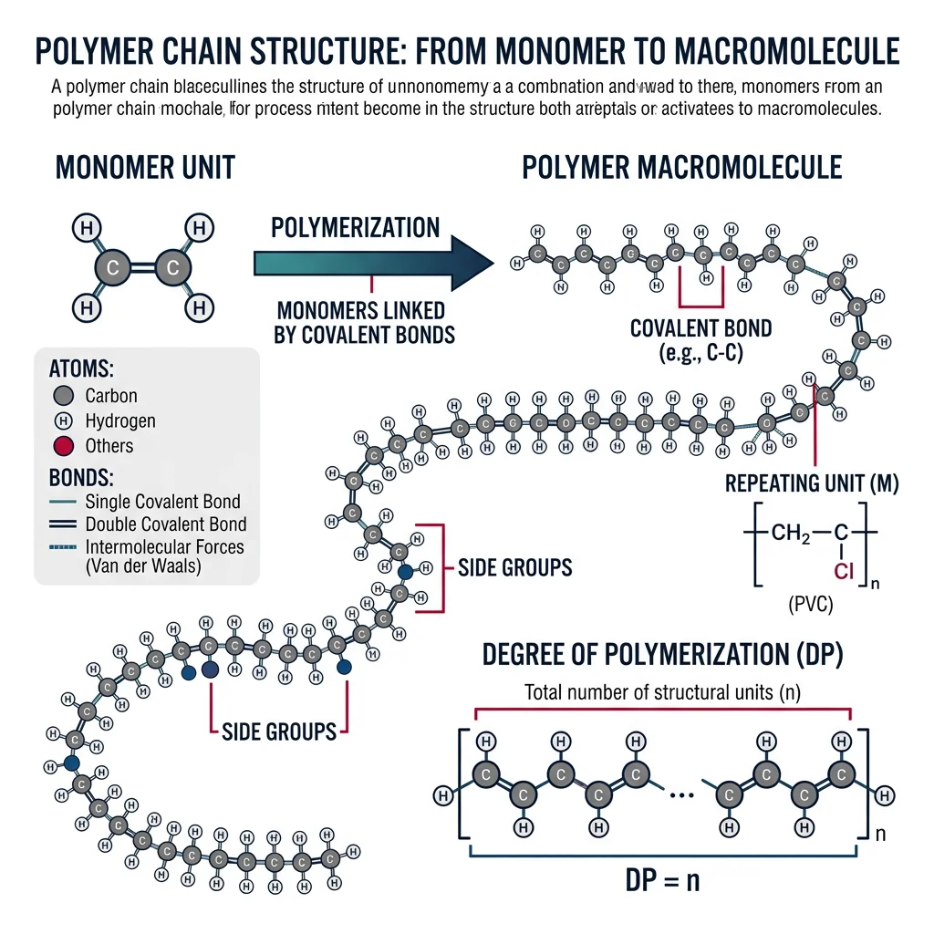
Imagine a single strand of spaghetti — that's a monomer. Now picture an entire plate of tangled spaghetti — that's a polymer. The word itself comes from the Greek poly (many) and meros (parts). Polymers are giant molecules — macromolecules — built by linking thousands or even millions of small repeating units called monomers through covalent bonds.

Polymers are arguably the most versatile class of materials on Earth. From the DNA in your cells to the plastic bottle on your desk, from Kevlar body armor to biodegradable surgical sutures, polymers dominate modern life. Understanding how they're built and how their molecular architecture determines their properties is the key to designing next-generation soft materials.

Polymerization Reactions

There are two fundamental routes from monomers to polymers:

1. Addition (Chain-Growth) Polymerization: Monomers add one at a time to a growing chain, typically via a reactive intermediate (free radical, cation, or anion). No by-products are released. The classic example is polyethylene — ethylene monomers ($\text{CH}_2\text{=CH}_2$) open their double bonds and link end-to-end.

2. Condensation (Step-Growth) Polymerization: Two different functional groups react, and a small molecule (usually water) is released as a by-product. Nylon 6,6 forms when a diamine reacts with a dicarboxylic acid, releasing $\text{H}_2\text{O}$ at every linkage.

Chain Architecture

The way polymer chains are connected determines their properties dramatically:

• Linear: Chains like parallel ropes. Can slide past each other → flexible, can crystallize. Example: HDPE (high-density polyethylene).
• Branched: Side chains prevent tight packing → lower density, lower crystallinity. Example: LDPE (low-density polyethylene).
• Crosslinked: Chains connected by covalent bridges → cannot melt or dissolve, elastic. Example: vulcanized rubber.
• Network: Extensive 3D crosslinking → rigid, strong, brittle. Example: epoxy resin, Bakelite.

Copolymers

When two or more different monomers are combined, the arrangement matters:

• Random copolymer: –A–B–A–A–B–A–B–B– (monomers in random order)
• Alternating copolymer: –A–B–A–B–A–B– (strict alternation)
• Block copolymer: –AAAA–BBBBB–AAAA– (long sequences of each)
• Graft copolymer: A backbone with B side chains (like a tree trunk with branches of a different species)

Tacticity

For vinyl polymers with a substituent group R on every other carbon, the spatial arrangement of those groups along the chain is called tacticity:

• Isotactic: All R groups on the same side → regular, crystallizable (e.g., isotactic polypropylene — stiff, high melting point)
• Syndiotactic: R groups strictly alternating sides → also regular, crystallizable
• Atactic: R groups randomly placed → irregular, amorphous (e.g., atactic polystyrene — clear, glassy)

import numpy as np

# Compute degree of polymerization from molecular weights
# Degree of polymerization: n = M_polymer / M_monomer

# Example: Polyethylene (PE)
# Monomer: ethylene C2H4, M0 = 28 g/mol
# Typical PE molecular weight: 200,000 g/mol

M_monomer = 28.0     # g/mol (ethylene)
M_polymer = 200000.0 # g/mol (polyethylene sample)

n = M_polymer / M_monomer
print(f"Monomer molecular weight: {M_monomer} g/mol")
print(f"Polymer molecular weight: {M_polymer:,.0f} g/mol")
print(f"Degree of polymerization (n): {n:,.0f}")
print(f"\nThis means ~{n:,.0f} ethylene units are linked together")
print(f"in a single polyethylene chain.")

# Compare different polymers
polymers = {
    "Polyethylene (PE)": (28, 200000),
    "Polystyrene (PS)": (104, 300000),
    "PVC": (62.5, 100000),
    "Nylon 6,6": (226, 30000),
    "PMMA": (100, 500000),
}

print(f"\n{'Polymer':<22} {'M_mono':>8} {'M_poly':>10} {'n':>8}")
print("-" * 52)
for name, (m0, mp) in polymers.items():
    dp = mp / m0
    print(f"{name:<22} {m0:>8.1f} {mp:>10,} {dp:>8,.0f}")

Molecular Weight Distribution

Unlike small molecules, polymers don't have a single molecular weight. A sample of polyethylene contains chains of many different lengths — some with 1,000 repeat units, others with 50,000. This spread is described by the molecular weight distribution.

Two key averages characterize this distribution:

Number-average molecular weight ($\bar{M}_n$): Counts each chain equally, regardless of size. Like a simple arithmetic mean of chain lengths:

$$\bar{M}_n = \frac{\sum N_i M_i}{\sum N_i}$$

Weight-average molecular weight ($\bar{M}_w$): Weights each chain by its mass. Larger chains contribute more. Always $\bar{M}_w \geq \bar{M}_n$:

$$\bar{M}_w = \frac{\sum N_i M_i^2}{\sum N_i M_i}$$

The ratio of these two averages is the polydispersity index (PDI or Đ):

$$\text{PDI} = \frac{\bar{M}_w}{\bar{M}_n} \geq 1$$

• PDI = 1: All chains identical length (monodisperse) — ideal but rare
• PDI ~ 1.5–2.0: Typical for condensation polymers
• PDI ~ 2–5: Common for free-radical addition polymers
• PDI > 20: Very broad distribution — poor mechanical properties

How is MW distribution measured? The gold standard is Gel Permeation Chromatography (GPC), also called Size Exclusion Chromatography (SEC). The polymer solution flows through a column packed with porous beads. Small chains enter the pores and take longer; large chains are excluded and elute first. A detector records the concentration vs. elution time, which is converted to a MW distribution curve.

import numpy as np
import matplotlib.pyplot as plt

# Simulate a molecular weight distribution (log-normal)
np.random.seed(42)

# Generate 10,000 polymer chains with log-normal MW distribution
mu = np.log(100000)   # Log of median MW
sigma = 0.6           # Breadth of distribution
molecular_weights = np.random.lognormal(mean=mu, sigma=sigma, size=10000)

# Calculate averages
Mn = np.mean(molecular_weights)                                    # Number-average
Mw = np.sum(molecular_weights**2) / np.sum(molecular_weights)      # Weight-average
PDI = Mw / Mn

print(f"Number-average MW (Mn): {Mn:,.0f} g/mol")
print(f"Weight-average MW (Mw): {Mw:,.0f} g/mol")
print(f"Polydispersity Index (PDI): {PDI:.2f}")

# Plot the distribution
fig, ax = plt.subplots(figsize=(9, 5))
ax.hist(molecular_weights / 1000, bins=80, density=True,
        alpha=0.7, color='#3B9797', edgecolor='white', linewidth=0.5)
ax.axvline(Mn/1000, color='#BF092F', linewidth=2, linestyle='--', label=f'Mn = {Mn/1000:.0f}k')
ax.axvline(Mw/1000, color='#132440', linewidth=2, linestyle='-',  label=f'Mw = {Mw/1000:.0f}k')
ax.set_xlabel('Molecular Weight (kg/mol)', fontsize=12)
ax.set_ylabel('Probability Density', fontsize=12)
ax.set_title(f'Molecular Weight Distribution (PDI = {PDI:.2f})', fontsize=14)
ax.legend(fontsize=11)
ax.set_xlim(0, 500)
plt.tight_layout()
plt.show()

Polymer Crystallinity

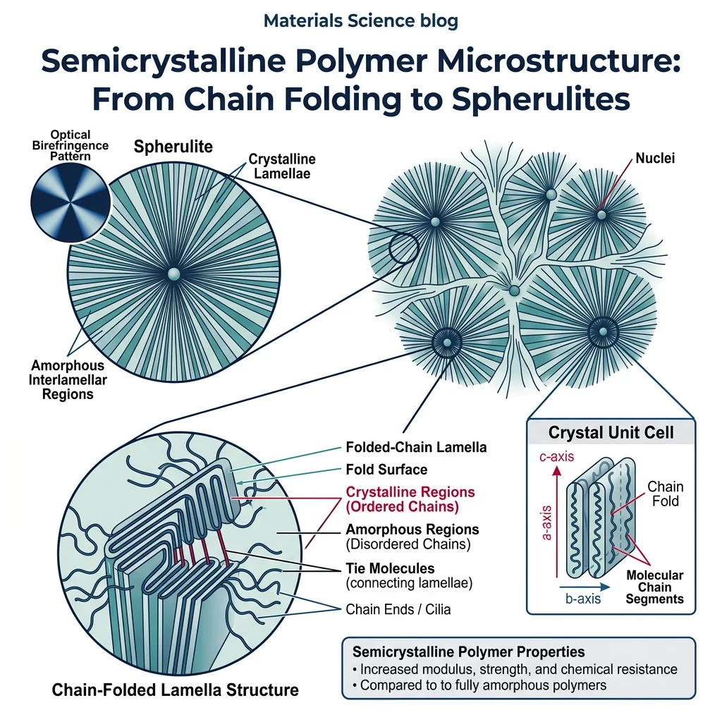
Most polymers are not fully crystalline or fully amorphous — they are semicrystalline. Imagine crumpling a bedsheet: some regions are neatly folded (crystalline), while others are tangled (amorphous). The fraction of crystalline material determines stiffness, density, transparency, and chemical resistance.

How do chains crystallize? Polymer chains fold back and forth to form flat plates called lamellae (typically 10–20 nm thick). These lamellae radiate outward from a central nucleus to form spherical structures called spherulites, visible under a polarized light microscope as beautiful Maltese-cross patterns. Think of it like folding a very long piece of paper accordion-style — the folds create an ordered, compact stack.

Factors Affecting Crystallinity

• Chain regularity: Simple, symmetric chains (PE, PTFE) crystallize easily. Bulky random side groups prevent it.
• Tacticity: Isotactic and syndiotactic polymers crystallize; atactic cannot.
• Cooling rate: Slow cooling allows time for chains to organize → higher crystallinity. Quenching freezes the amorphous state.
• Drawing/stretching: Mechanically aligning chains promotes crystallization (strain-induced crystallization).
• Molecular weight: Very high MW chains entangle more → harder to crystallize, but once crystallized they're tougher.

DSC Measurement: Differential Scanning Calorimetry measures the heat flow as a polymer is heated. The area of the melting peak, compared to a 100% crystalline reference, gives the percent crystallinity: $\%\ \text{crystallinity} = \frac{\Delta H_m}{\Delta H_m^0} \times 100$

Polymer Classifications

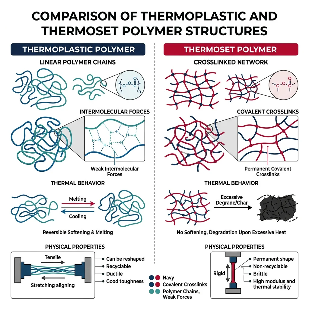
The most fundamental division in polymer science is between the two great families: thermoplastics and thermosets.

Think of it like cooking. Chocolate is a thermoplastic — you can melt it, pour it into a mold, let it solidify, then remelt it and reshape it as many times as you like. An egg, once cooked, is a thermoset — the proteins have permanently crosslinked, and no amount of heating will turn it back into a raw egg.

Common Thermoplastics

• PE (polyethylene): Most produced plastic in the world — bags, bottles, pipes
• PP (polypropylene): Living hinge packaging, automotive, textiles
• PS (polystyrene): Disposable cutlery, insulation foam (Styrofoam)
• PVC (polyvinyl chloride): Pipes, window frames, flooring
• PET (polyethylene terephthalate): Drink bottles, polyester clothing
• PMMA (poly(methyl methacrylate)): Plexiglass, optical lenses
• PC (polycarbonate): Bulletproof glass, safety goggles, CDs
• Nylon (polyamide): Gears, bearings, textiles, zip ties
• PTFE (Teflon): Non-stick coatings, seals, chemical-resistant linings

Common Thermosets

• Epoxy: Adhesives, composite matrices (carbon fiber), coatings
• Phenolic (Bakelite): The first synthetic plastic — electrical insulators, pot handles
• Unsaturated polyester: Fiberglass boats, bath tubs, automotive body panels
• Polyurethane: Foams (mattresses, insulation), coatings, elastomers
• Silicone: Sealants, medical implants, cookware, lubricants

Properties Comparison

Property	Thermoplastics	Thermosets
Melting behavior	Soften and flow on heating	Do not melt — decompose
Recyclability	Recyclable (remelt)	Not easily recyclable
Crosslinks	None (physical entanglements)	Extensive covalent crosslinks
Solubility	Dissolve in appropriate solvents	Insoluble (swell at most)
Creep resistance	Poor to moderate	Excellent
Processing	Injection molding, extrusion, thermoforming	Casting, compression molding, RTM
Typical cost	Low to moderate	Moderate to high

Elastomers & Rubbers

Elastomers are a special class of polymers that can stretch to several times their original length and snap back when released. But what makes rubber stretchy? The answer is beautifully counterintuitive — it's driven by entropy, not energy.

In an unstretched rubber band, the polymer chains are randomly coiled — a high-entropy, disordered state. When you stretch the rubber, chains are forced to align — a low-entropy, ordered state. Thermodynamics demands that the system return to maximum entropy, so the chains pull back to their coiled configuration. The restoring force is essentially entropy trying to increase.

Natural vs Synthetic Rubber

• Natural rubber (NR): Polyisoprene harvested from Hevea brasiliensis trees. Excellent elasticity, poor heat and oil resistance.
• SBR (styrene-butadiene rubber): The most-produced synthetic rubber — car tires, shoe soles.
• NBR (nitrile rubber): Oil-resistant — gaskets, seals, gloves for automotive and chemical use.
• Silicone rubber: Temperature-stable from –60°C to +230°C — medical devices, cookware, aerospace seals.
• EPDM: Weather-resistant — automotive weatherstripping, roofing membranes.

Glass Transition Temperature

If you could pick just one number to characterize a polymer, it would be its glass transition temperature ($T_g$). This is the temperature below which polymer chains are frozen in place (glassy, rigid, brittle) and above which they gain enough thermal energy to wriggle and slide (rubbery, flexible, tough).

$T_g$ is not a melting point — it's a transition in the amorphous regions. Think of honey: cold honey is stiff (glassy); warm honey flows (rubbery). The transition is gradual, occurring over a range of ~10–30°C.

What Shifts $T_g$?

• Backbone flexibility: Flexible chains (Si–O in silicones) → low $T_g$. Rigid chains (aromatic rings in polycarbonate) → high $T_g$.
• Bulky side groups: Large pendant groups restrict rotation → higher $T_g$ (e.g., PS has $T_g$ = 100°C due to phenyl groups).
• Polar interactions: Strong intermolecular forces (hydrogen bonds in nylon) → higher $T_g$.
• Crosslinking: More crosslinks restrict chain mobility → higher $T_g$.
• Plasticizers: Small molecules that slip between chains and push them apart → lower $T_g$ (this is how rigid PVC becomes flexible PVC).

import numpy as np
import matplotlib.pyplot as plt

# Model the elastic modulus vs temperature showing glass transition
# Using a sigmoid function to approximate the Tg transition

def modulus_vs_temp(T, Tg, E_glassy=3e9, E_rubbery=1e6, width=15):
    """Approximate modulus (Pa) as a function of temperature.
    Sigmoid transition centered at Tg."""
    return E_rubbery + (E_glassy - E_rubbery) / (1 + np.exp((T - Tg) / width))

# Temperature range
T = np.linspace(-150, 250, 500)

# Three polymers with different Tg values
polymers = {
    'Polyethylene (Tg = -120°C)': -120,
    'PET (Tg = 70°C)': 70,
    'Polycarbonate (Tg = 150°C)': 150,
}
colors = ['#3B9797', '#BF092F', '#132440']

fig, ax = plt.subplots(figsize=(10, 6))
for (name, tg), color in zip(polymers.items(), colors):
    E = modulus_vs_temp(T, tg)
    ax.semilogy(T, E, linewidth=2.5, color=color, label=name)
    ax.axvline(tg, color=color, linestyle=':', alpha=0.5)

ax.axvline(25, color='gray', linestyle='--', alpha=0.6, label='Room Temp (25°C)')
ax.set_xlabel('Temperature (°C)', fontsize=12)
ax.set_ylabel('Elastic Modulus (Pa)', fontsize=12)
ax.set_title('Glass Transition: Modulus vs Temperature', fontsize=14)
ax.set_ylim(1e5, 1e10)
ax.legend(fontsize=10, loc='upper right')
ax.grid(True, alpha=0.3)
plt.tight_layout()
plt.show()

Mechanical Behavior

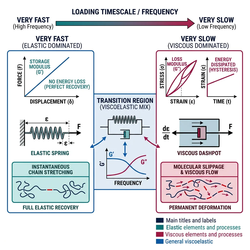
Polymers are neither purely elastic (like a steel spring) nor purely viscous (like honey). They are viscoelastic — their response depends on both the magnitude of the force and how fast it is applied. This dual nature is what makes polymers both fascinating and tricky to engineer with.

The classic demonstration is Silly Putty: throw it at a wall and it bounces (elastic response to fast loading); pull it slowly and it stretches and flows (viscous response to slow loading); leave a ball of it on a table overnight and it flattens under its own weight (creep).

Mechanical Models

Engineers use combinations of springs (elastic element, modulus $E$) and dashpots (viscous element, viscosity $\eta$) to model viscoelastic behavior:

Maxwell Model (spring + dashpot in series): Good for modeling stress relaxation — apply a constant strain and watch the stress decay exponentially over time. The relaxation time is $\tau = \eta / E$.

$$\sigma(t) = \sigma_0 \, e^{-t/\tau}$$

Kelvin-Voigt Model (spring + dashpot in parallel): Good for modeling creep — apply a constant stress and watch the strain increase gradually toward an equilibrium value.

$$\varepsilon(t) = \frac{\sigma_0}{E}\left(1 - e^{-t/\tau}\right)$$

import numpy as np
import matplotlib.pyplot as plt

# Maxwell Model: Stress Relaxation
# sigma(t) = sigma_0 * exp(-t / tau)
# tau = eta / E (relaxation time)

E = 1e9       # Elastic modulus (Pa) — 1 GPa, typical glassy polymer
eta = 1e12    # Viscosity (Pa·s)
tau = eta / E # Relaxation time (seconds)
sigma_0 = 10e6  # Initial stress (Pa) — 10 MPa

t = np.linspace(0, 5 * tau, 500)
sigma = sigma_0 * np.exp(-t / tau)

fig, (ax1, ax2) = plt.subplots(1, 2, figsize=(13, 5))

# Plot 1: Stress relaxation (Maxwell)
ax1.plot(t / tau, sigma / 1e6, linewidth=2.5, color='#BF092F')
ax1.axhline(sigma_0 / 1e6 / np.e, color='gray', linestyle='--', alpha=0.6,
            label=f'σ₀/e at t = τ = {tau:.0f} s')
ax1.set_xlabel('Time (t / τ)', fontsize=12)
ax1.set_ylabel('Stress (MPa)', fontsize=12)
ax1.set_title('Maxwell Model: Stress Relaxation', fontsize=13)
ax1.legend(fontsize=10)
ax1.grid(True, alpha=0.3)

# Plot 2: Creep (Kelvin-Voigt model)
# epsilon(t) = (sigma_0 / E) * (1 - exp(-t / tau))
sigma_applied = 5e6  # Applied constant stress (Pa)
epsilon = (sigma_applied / E) * (1 - np.exp(-t / tau))

ax2.plot(t / tau, epsilon * 100, linewidth=2.5, color='#3B9797')
ax2.axhline((sigma_applied / E) * 100, color='gray', linestyle='--', alpha=0.6,
            label=f'Equilibrium strain = {sigma_applied/E*100:.4f}%')
ax2.set_xlabel('Time (t / τ)', fontsize=12)
ax2.set_ylabel('Strain (%)', fontsize=12)
ax2.set_title('Kelvin-Voigt Model: Creep', fontsize=13)
ax2.legend(fontsize=10)
ax2.grid(True, alpha=0.3)

plt.tight_layout()
plt.show()

print(f"Relaxation time τ = η/E = {eta:.0e} / {E:.0e} = {tau:.0f} seconds")
print(f"At t = τ, stress drops to σ₀/e ≈ {sigma_0/np.e/1e6:.2f} MPa (37% of initial)")

Rheology & Flow Behavior

Rheology is the science of flow and deformation. For polymer processing — extrusion, injection molding, blow molding, 3D printing — understanding how a polymer melt flows under different conditions is absolutely critical.

Newtonian vs Non-Newtonian Fluids

A Newtonian fluid (water, simple oils) has a constant viscosity regardless of how fast you shear it: $\tau = \eta \dot{\gamma}$ where $\tau$ is shear stress, $\eta$ is viscosity, and $\dot{\gamma}$ is shear rate. Most polymer melts are non-Newtonian.

Shear-thinning (pseudoplastic): Viscosity decreases with increasing shear rate. This is by far the most common behavior in polymer melts and solutions. Under high shear, entangled chains align in the flow direction and disentangle, reducing resistance. Real-world examples: ketchup (won't flow until you shake it), paint (flows smoothly under a brush but doesn't drip off the wall).

Shear-thickening (dilatant): Viscosity increases with shear rate. Much rarer but spectacular. The classic example is oobleck — a cornstarch-water suspension that you can walk on if you run, but sink into if you stand still. Under sudden impact, particles jam together and the suspension locks up.

The power-law model captures both behaviors:

$$\tau = K \dot{\gamma}^n$$

where $K$ is the consistency index and $n$ is the flow behavior index. For shear-thinning, $n < 1$; for Newtonian, $n = 1$; for shear-thickening, $n > 1$.

Melt Flow Index (MFI): A practical polymer processing measurement — the mass (in grams) of polymer melt that flows through a standard die under a standard load in 10 minutes. High MFI = easy flow (good for thin-wall injection molding). Low MFI = high viscosity (good for blow molding, where you need the melt to hold its shape).

import numpy as np
import matplotlib.pyplot as plt

# Power-law fluid model: tau = K * gamma_dot^n
# Plot viscosity vs shear rate for different fluid types

gamma_dot = np.logspace(-1, 3, 200)  # Shear rate (1/s)

K = 100  # Consistency index (Pa·s^n)

# Different flow behavior indices
fluids = {
    'Shear-thinning (n=0.3)': 0.3,
    'Shear-thinning (n=0.6)': 0.6,
    'Newtonian (n=1.0)': 1.0,
    'Shear-thickening (n=1.4)': 1.4,
}
colors = ['#BF092F', '#16476A', '#3B9797', '#132440']

fig, (ax1, ax2) = plt.subplots(1, 2, figsize=(13, 5))

for (name, n), color in zip(fluids.items(), colors):
    tau = K * gamma_dot**n
    eta_apparent = K * gamma_dot**(n - 1)  # Apparent viscosity
    ax1.loglog(gamma_dot, tau, linewidth=2.5, color=color, label=name)
    ax2.loglog(gamma_dot, eta_apparent, linewidth=2.5, color=color, label=name)

ax1.set_xlabel('Shear Rate (1/s)', fontsize=12)
ax1.set_ylabel('Shear Stress (Pa)', fontsize=12)
ax1.set_title('Shear Stress vs Shear Rate', fontsize=13)
ax1.legend(fontsize=9)
ax1.grid(True, alpha=0.3)

ax2.set_xlabel('Shear Rate (1/s)', fontsize=12)
ax2.set_ylabel('Apparent Viscosity (Pa·s)', fontsize=12)
ax2.set_title('Viscosity vs Shear Rate', fontsize=13)
ax2.legend(fontsize=9)
ax2.grid(True, alpha=0.3)

plt.tight_layout()
plt.show()

print("Shear-thinning (n < 1): Viscosity DECREASES with shear rate")
print("  → Most polymer melts, ketchup, paint, blood")
print("Newtonian (n = 1): Viscosity is CONSTANT")
print("  → Water, simple oils, dilute solutions")
print("Shear-thickening (n > 1): Viscosity INCREASES with shear rate")
print("  → Cornstarch suspensions (oobleck), some ceramic slurries")

Polymer Degradation

All polymers degrade over time. Understanding degradation mechanisms is essential for predicting service life, designing stabilizer packages, and — increasingly — engineering controlled degradation for biodegradable materials.

Thermal Degradation

At elevated temperatures, polymer chains break apart via two main mechanisms:

• Random chain scission: Bonds break at random positions along the backbone. Molecular weight drops rapidly but monomer yield is low. Common in polyethylene and polypropylene — they become waxy and weak.
• Depolymerization (unzipping): The chain breaks apart from the end, regenerating monomer units one at a time. PMMA (acrylic) depolymerizes almost quantitatively above 300°C — which is why it can be chemically recycled by pyrolysis.

UV Degradation

Ultraviolet light provides enough energy (~300-400 kJ/mol for UV-A, more for UV-B) to break C–C and C–H bonds in polymer chains. This generates free radicals that initiate oxidative chain reactions. The result: yellowing, embrittlement, and cracking. Polypropylene is especially susceptible — outdoor PP products always contain UV stabilizers (HALS — hindered amine light stabilizers).

Oxidative Degradation

Oxygen reacts with free radicals on polymer chains to form peroxides and hydroperoxides, which decompose to generate more radicals — an autocatalytic chain reaction. Antioxidants (e.g., Irganox 1010, BHT) are added as sacrificial radical scavengers to break this cycle.

Hydrolytic Degradation

Polymers with hydrolyzable bonds (esters, amides, anhydrides) can be cleaved by water, especially in acidic or basic conditions. This is undesirable in nylon car parts exposed to moisture, but intentionally designed into biodegradable polymers like PLA (polylactic acid) and PGA (polyglycolic acid) used in absorbable surgical sutures.

Environmental Stress Cracking

Some polymers crack under combined mechanical stress and chemical exposure, even though neither alone would cause failure. HDPE bottles can crack when exposed to certain detergents under stress. Polycarbonate is sensitive to acetone and alkaline cleaners.

Biopolymers & Frontier Research

Nature invented polymers billions of years before we did. Biopolymers — polymers produced by living organisms — include some of the most remarkable materials known:

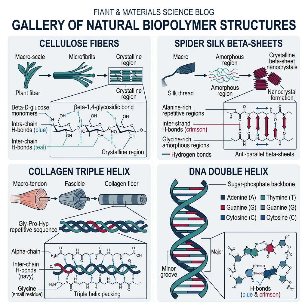
• Cellulose: The most abundant organic polymer on Earth. Every plant cell wall is made of cellulose — a linear chain of glucose units. Wood, cotton, and paper are cellulose-based.
• Chitin: The second most abundant biopolymer — found in insect exoskeletons, crustacean shells, and fungal cell walls.
• Silk: Spider dragline silk has a tensile strength of ~1.3 GPa — stronger than steel per unit weight — achieved through alternating crystalline β-sheet domains and amorphous flexible regions.
• Collagen: The most abundant protein in mammals (25–35% of total body protein). Its triple-helix structure provides tensile strength to skin, tendons, bones, and blood vessels.
• DNA: A double-stranded helical polymer of nucleotides — perhaps the most important polymer in existence, encoding the instructions for life itself.

Bioplastics

The growing urgency around plastic pollution has driven enormous interest in bio-based and biodegradable plastics:

• PLA (polylactic acid): Made from fermented corn starch or sugarcane. Compostable in industrial facilities (~60°C). Widely used in 3D printing and food packaging.
• PHA (polyhydroxyalkanoates): Produced by bacteria as energy storage granules. Truly biodegradable in soil and marine environments — but expensive.
• PBS (polybutylene succinate): Bio-based and compostable. Used in mulch films and food packaging.

Recycling: Mechanical vs Chemical

The circular economy for polymers depends on effective recycling:

• Mechanical recycling: Shred → wash → melt → repellet. Works well for clean, sorted single-polymer waste (PET bottles, HDPE containers). Each cycle degrades molecular weight slightly, limiting the number of reuse cycles.
• Chemical recycling: Break polymer back down to monomers or feedstock using pyrolysis, glycolysis, or enzymatic processes. Produces virgin-quality material but requires more energy. PET glycolysis and PMMA depolymerization are commercially viable.

Self-Healing Polymers

Imagine a material that repairs itself when damaged — like human skin healing a cut. Self-healing polymers are making this science-fiction concept a reality, and they broadly fall into two categories:

Extrinsic Self-Healing

Healing agents are pre-loaded into the material. When a crack forms, it ruptures the containers and releases the healing agent.

• Microcapsule approach (White et al., 2001): The landmark paper in Nature embedded micro-capsules filled with dicyclopentadiene (DCPD) monomer into an epoxy matrix, along with Grubbs' catalyst dispersed in the matrix. When a crack ruptured the capsules, DCPD flowed into the crack and polymerized on contact with the catalyst, rebonding the surfaces. Recovery of ~75% of original fracture toughness was demonstrated.
• Vascular networks: Instead of capsules (one-shot healing), hollow channels carry healing agent continuously — like blood vessels. Enables multiple healing events at the same location.

Intrinsic Self-Healing

The polymer itself has reversible bonds that can reform after breaking — no capsules or channels needed.

• Diels-Alder (DA) reversible crosslinks: Furan and maleimide groups form covalent bonds at room temperature but break apart at ~120°C (retro-DA reaction). Heat the damaged part → bonds break → chains become mobile → cool down → bonds reform. Fully reversible and repeatable.
• Supramolecular polymers: Chains held together by hydrogen bonds, metal-ligand coordination, or π-π stacking instead of covalent bonds. These non-covalent bonds are individually weak but collectively strong, and they can re-form spontaneously at room temperature.
• Vitrimers: Thermoset-like polymers with exchangeable crosslinks. At elevated temperature, bonds rearrange (associative exchange) without net loss of crosslinks — the material can be reshaped like a thermoplastic while maintaining thermoset-like mechanical properties.

Conductive & Biodegradable Polymers

For most of polymer history, the assumption was simple: polymers are insulators. Polyethylene insulates electrical cables; PVC coats wires; rubber gloves protect electricians. Then, in 1977, three chemists — Alan Heeger, Alan MacDiarmid, and Hideki Shirakawa — discovered that polyacetylene, when doped with iodine vapor, becomes as conductive as some metals. This discovery earned them the 2000 Nobel Prize in Chemistry.

How Do Polymers Conduct?

Conjugated polymers have alternating single and double bonds along their backbone (–C=C–C=C–). This creates a continuous system of overlapping p-orbitals — a "highway" for electrons. In their pristine state, these polymers are semiconductors. Chemical or electrochemical doping — adding or removing electrons — converts them into conductors.

Key conducting polymers:

• Polyacetylene: The original — high conductivity when doped, but unstable in air
• PEDOT:PSS: The workhorse of organic electronics — transparent, flexible, processable from water. Used in almost every OLED display and organic solar cell as a hole-transport layer.
• Polyaniline (PANI): Easy to synthesize, tunable conductivity, anti-corrosion coatings
• Polypyrrole (PPy): Biocompatible — used in neural interfaces and biosensors
• Polythiophenes (P3HT): Organic solar cell active layers

Applications

• Flexible OLEDs: Your phone's curved display uses organic semiconducting polymers as light-emitting layers. Polymer OLEDs can be printed using inkjet technology — enabling roll-to-roll manufacturing of displays.
• Organic solar cells: Semiconducting polymers mixed with fullerene or non-fullerene acceptors create bulk heterojunction solar cells — flexible, lightweight, and manufacturable at low cost. Efficiencies now exceed 19%.
• Wearable sensors: Conductive polymer films on flexible substrates can detect strain, pressure, temperature, and chemical analytes — enabling e-skin for prosthetics and health monitoring.
• Thermoelectric generators: PEDOT-based polymers can convert waste heat to electricity — low efficiency but ultra-low cost and flexible.

Biodegradable Polymers for Packaging: Degradation Timeline

How long do common polymers take to degrade in the environment?

Material	Degradation Time	Notes
Paper bag	1–3 months	Cellulose — readily biodegradable
PHA packaging	3–6 months	Biodegradable in soil and marine
PLA cup	6–24 months	Only in industrial composting (>58°C)
Nylon fabric	30–40 years	Slow hydrolytic and microbial attack
HDPE bottle	100+ years	UV degradation → fragmentation → microplastics
PET bottle	400+ years	Extremely resistant to biodegradation
PS (Styrofoam)	500+ years	Essentially permanent in landfills

Exercises & Applications

Test your understanding of polymers and soft materials with these practice problems. Work through them to reinforce the concepts covered in this article.

Conclusion & Next Steps

Polymers are the most diverse and versatile class of engineering materials. From single monomers, nature and chemists build macromolecules whose properties span an astonishing range — from ultra-soft hydrogels to bulletproof Kevlar fibers, from insulating cable coatings to conducting polymer LEDs, from permanent thermoset adhesives to self-healing coatings that repair themselves in sunlight.

The key themes connecting everything in this guide are: molecular architecture determines properties (linear vs branched vs crosslinked, tacticity, copolymer arrangement), time and temperature matter ($T_g$ governs whether a polymer is glassy or rubbery; viscoelastic models capture time-dependent behavior), and sustainability is driving innovation (biopolymers, chemical recycling, vitrimers, and self-healing materials are reshaping the polymer landscape).

In the next installment, we shift from soft materials to hard ones — and discover how ceramics, glasses, and composite materials combine the best properties of multiple material classes to achieve performance that no single material can match alone.