We use cookies to enhance your browsing experience, serve personalized content, and analyze our traffic.
By clicking "Accept All", you consent to our use of cookies. See our
Privacy Policy
for more information.
A database is an organized collection of structured data that can be easily accessed, managed, and updated. Think of it as a digital filing cabinet—but infinitely more powerful, capable of handling millions of records with lightning-fast queries.
Series Context: This is Part 1 of 15 in the Complete Database Mastery series. We're building your database skills from absolute fundamentals to architect-level expertise.
Imagine a massive library with millions of books. Without any organization system, finding a specific book would take forever. Libraries solve this with:
Catalogs — Quick lookup of book locations (like database indexes)
Shelves — Physical storage organized by category (like rows)
Librarians — People who manage access and organization (like the DBMS)
A database works exactly the same way—it organizes data so you can find any piece of information in milliseconds, even among billions of records.
Why Learn SQL? SQL (Structured Query Language) is the universal language for talking to databases. Over 50 years old and still the #1 skill employers seek in data professionals. Whether you're building web apps, analyzing data, or managing systems—SQL is essential.
Real-World Database Applications
Databases power virtually every digital service you use:
E-Commerce (Amazon, Shopify)
Product catalogs, customer accounts, orders, inventory, reviews—all stored in databases. When you search for "wireless headphones," a database query returns matching products in milliseconds.
Social Media (Facebook, Twitter)
User profiles, posts, comments, likes, friend connections—billions of records queried millions of times per second. Your news feed is generated by complex database queries.
Banking & Finance
Account balances, transactions, loans, interest calculations—all require databases with absolute accuracy and reliability. A single wrong query could move millions incorrectly.
Database Concepts
Before writing any SQL, you need to understand the building blocks of database systems. These concepts form the foundation for everything that follows.
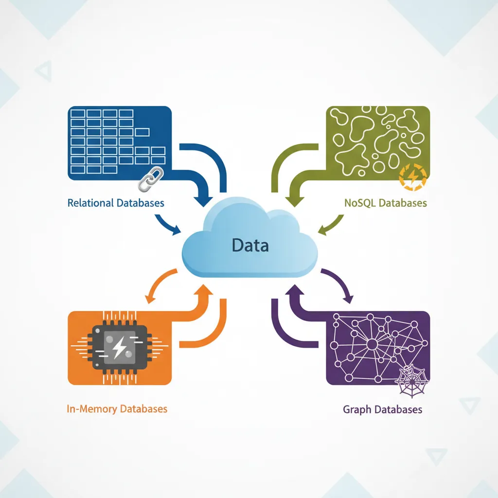
Overview of database system types: relational, NoSQL, in-memory, and graph databases
DBMS vs RDBMS
A Database Management System (DBMS) is software that manages databases—it handles storage, retrieval, and manipulation of data. Think of it as the operating system for your data.
Types of Database Systems
Type
Description
Examples
RDBMS
Relational databases using tables with rows and columns, linked by relationships
PostgreSQL, MySQL, SQL Server, Oracle
NoSQL
Non-relational databases for flexible, unstructured data
MongoDB, Cassandra, DynamoDB
In-Memory
Data stored in RAM for ultra-fast access
Redis, Memcached
Graph
Optimized for connected data and relationships
Neo4j, Amazon Neptune
In this series, we focus primarily on RDBMS (Relational Database Management Systems) because:
They power 70%+ of enterprise applications
SQL skills transfer across all relational databases
They provide strong data integrity guarantees
Most interview questions focus on relational databases
Tables, Rows & Columns
In relational databases, data is organized into tables—also called relations. Each table represents a specific entity (customers, products, orders).
The Spreadsheet Analogy: If you've used Excel, you already understand tables! A database table is like a spreadsheet where columns define what data you store (name, email, age) and each row is one record (one customer, one product).
Here's an example employees table:
-- Conceptual view of an employees table
+----+------------+-----------+------------+--------+
| id | first_name | last_name | department | salary |
+----+------------+-----------+------------+--------+
|  1 | John       | Smith     | Engineering| 75000  |
|  2 | Sarah      | Johnson   | Marketing  | 65000  |
|  3 | Mike       | Williams  | Engineering| 80000  |
|  4 | Emily      | Brown     | HR         | 55000  |
+----+------------+-----------+------------+--------+
Key terminology:
Column (Field/Attribute) — A single piece of data type (id, first_name, salary)
Row (Record/Tuple) — One complete entry in the table (one employee)
Cell — The intersection of a row and column (John's salary: 75000)
Schema — The structure definition (column names, data types, constraints)
Primary Keys
A Primary Key is a column (or combination of columns) that uniquely identifies each row in a table. Like a social security number for your data—no two rows can have the same primary key value.
-- Creating a table with a primary key
CREATE TABLE employees (
    id INT PRIMARY KEY,           -- 'id' uniquely identifies each employee
    first_name VARCHAR(50),
    last_name VARCHAR(50),
    email VARCHAR(100) UNIQUE,    -- emails must also be unique
    department VARCHAR(50),
    salary DECIMAL(10, 2)
);
Primary Key Best Practices
Use surrogate keys — Auto-incrementing integers (id) rather than natural keys (email)
Keep them simple — Single column when possible, avoid composite keys unless necessary
Never change them — Primary keys should be immutable; changing them breaks relationships
Consider UUIDs — For distributed systems where auto-increment causes conflicts
-- Auto-incrementing primary key (PostgreSQL)
CREATE TABLE products (
    id SERIAL PRIMARY KEY,        -- Auto-increments: 1, 2, 3, ...
    name VARCHAR(100) NOT NULL,
    price DECIMAL(10, 2) NOT NULL,
    created_at TIMESTAMP DEFAULT CURRENT_TIMESTAMP
);

-- Auto-incrementing primary key (MySQL)
CREATE TABLE products (
    id INT AUTO_INCREMENT PRIMARY KEY,
    name VARCHAR(100) NOT NULL,
    price DECIMAL(10, 2) NOT NULL,
    created_at TIMESTAMP DEFAULT CURRENT_TIMESTAMP
);
Basic SQL Statements (CRUD Operations)
CRUD stands for Create, Read, Update, Delete—the four fundamental operations you perform on any database. Master these, and you can manipulate any data.
The four fundamental CRUD operations mapped to SQL statements: INSERT, SELECT, UPDATE, DELETE
SQL Syntax Note: SQL keywords are case-insensitive (SELECT = select = SeLeCt), but the convention is UPPERCASE for keywords and lowercase for table/column names. This improves readability.
SELECT Queries (Read)
The SELECT statement retrieves data from one or more tables. It's the most commonly used SQL command—you'll write hundreds of SELECT queries for every INSERT.
-- Basic SELECT: Get all columns from a table
SELECT * FROM employees;

-- Select specific columns
SELECT first_name, last_name, salary FROM employees;

-- Select with column aliases (rename output columns)
SELECT
    first_name AS "First Name",
    last_name AS "Last Name",
    salary AS "Annual Salary"
FROM employees;

-- Select with expressions (calculated columns)
SELECT
    first_name,
    last_name,
    salary,
    salary * 12 AS annual_salary,
    salary * 0.20 AS tax_deduction
FROM employees;
Pro Tip: Avoid SELECT *
While SELECT * is convenient for exploration, avoid it in production code:
Returns unnecessary data, wasting bandwidth and memory
Breaks when table schema changes (new columns added)
Makes code harder to understand—which columns are actually needed?
Always specify the columns you need.
INSERT Statements (Create)
The INSERT statement adds new rows to a table. You can insert one row at a time or multiple rows in a single statement.
-- Insert a single row (specifying columns)
INSERT INTO employees (first_name, last_name, department, salary)
VALUES ('Alice', 'Chen', 'Engineering', 90000);

-- Insert with all columns (column list optional if providing all values)
INSERT INTO employees
VALUES (5, 'Bob', 'Miller', 'Sales', 60000);

-- Insert multiple rows at once (much faster than individual inserts!)
INSERT INTO employees (first_name, last_name, department, salary)
VALUES
    ('Carol', 'Davis', 'Marketing', 70000),
    ('David', 'Lee', 'Engineering', 85000),
    ('Eve', 'Wilson', 'HR', 58000);

-- Insert with a subquery (copy data from another table)
INSERT INTO employees_backup (first_name, last_name, department, salary)
SELECT first_name, last_name, department, salary
FROM employees
WHERE department = 'Engineering';
UPDATE Statements (Update)
The UPDATE statement modifies existing rows. Always use a WHERE clause—without it, you'll update every row in the table!
-- Update a single row
UPDATE employees
SET salary = 95000
WHERE id = 1;

-- Update multiple columns
UPDATE employees
SET
    department = 'Senior Engineering',
    salary = salary * 1.10  -- 10% raise
WHERE id = 3;

-- Update multiple rows matching a condition
UPDATE employees
SET salary = salary * 1.05  -- 5% raise for everyone in Engineering
WHERE department = 'Engineering';

-- Update with a calculated value
UPDATE products
SET price = price * 0.90  -- 10% discount
WHERE category = 'Clearance';
DANGER: Always Test with SELECT First! Before running an UPDATE, run the WHERE clause as a SELECT to verify which rows will be affected:
-- First: Check which rows will be updated
SELECT * FROM employees WHERE department = 'Engineering';

-- Then: Run the UPDATE
UPDATE employees SET salary = salary * 1.05 WHERE department = 'Engineering';
DELETE Statements (Delete)
The DELETE statement removes rows from a table. Like UPDATE, always use WHERE to avoid deleting everything.
-- Delete a specific row
DELETE FROM employees
WHERE id = 5;

-- Delete multiple rows matching a condition
DELETE FROM employees
WHERE department = 'Contractors' AND hire_date < '2020-01-01';

-- Delete all rows (but keep the table structure)
DELETE FROM temp_logs;

-- TRUNCATE: Faster way to delete all rows (can't use WHERE, resets auto-increment)
TRUNCATE TABLE temp_logs;
DELETE vs TRUNCATE vs DROP
Command
What It Does
Can Rollback?
WHERE Clause?
DELETE
Removes specific rows
Yes ✓
Yes ✓
TRUNCATE
Removes all rows (fast)
No ✗
No ✗
DROP TABLE
Removes entire table
No ✗
N/A
Filtering & Sorting
Most queries don't return all rows—you filter to find exactly what you need. SQL provides powerful tools for narrowing results and organizing output.
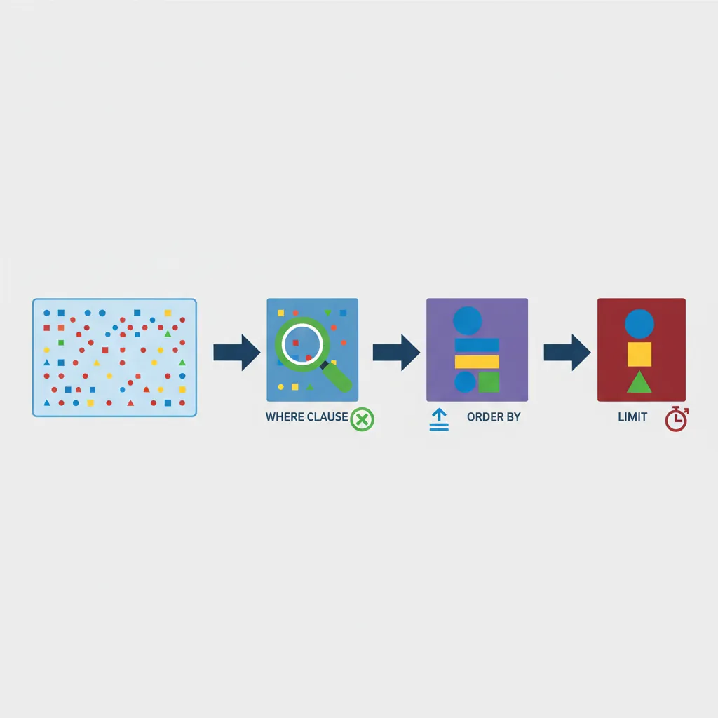
SQL query filtering pipeline: WHERE narrows rows, ORDER BY sorts results, LIMIT caps output
WHERE Clause
The WHERE clause filters rows based on conditions. Only rows that satisfy all conditions are returned.
-- Basic comparison operators
SELECT * FROM employees WHERE salary > 70000;
SELECT * FROM employees WHERE department = 'Engineering';
SELECT * FROM employees WHERE salary >= 60000 AND salary <= 80000;

-- Not equal (both syntaxes work)
SELECT * FROM employees WHERE department != 'HR';
SELECT * FROM employees WHERE department <> 'HR';

-- NULL handling (use IS NULL, not = NULL)
SELECT * FROM employees WHERE manager_id IS NULL;
SELECT * FROM employees WHERE phone IS NOT NULL;

-- Pattern matching with LIKE
SELECT * FROM employees WHERE first_name LIKE 'J%';      -- Starts with J
SELECT * FROM employees WHERE last_name LIKE '%son';     -- Ends with 'son'
SELECT * FROM employees WHERE email LIKE '%@gmail.com';  -- Gmail addresses
SELECT * FROM employees WHERE first_name LIKE '_o_n';    -- 4 chars, 'o' in 2nd, 'n' in 4th

-- IN operator (matches any value in list)
SELECT * FROM employees
WHERE department IN ('Engineering', 'Marketing', 'Sales');

-- BETWEEN operator (inclusive range)
SELECT * FROM employees
WHERE salary BETWEEN 50000 AND 80000;

-- Same as:
SELECT * FROM employees
WHERE salary >= 50000 AND salary <= 80000;
Combining Conditions: AND, OR, NOT
-- AND: Both conditions must be true
SELECT * FROM employees
WHERE department = 'Engineering' AND salary > 75000;

-- OR: At least one condition must be true
SELECT * FROM employees
WHERE department = 'Engineering' OR department = 'Sales';

-- NOT: Negates a condition
SELECT * FROM employees
WHERE NOT department = 'HR';

-- Complex conditions (use parentheses for clarity!)
SELECT * FROM employees
WHERE (department = 'Engineering' OR department = 'Sales')
  AND salary > 60000
  AND hire_date >= '2023-01-01';
ORDER BY
The ORDER BY clause sorts results. By default, sorting is ascending (A-Z, 0-9). Use DESC for descending order.
-- Sort by salary (ascending - lowest first)
SELECT first_name, last_name, salary
FROM employees
ORDER BY salary;

-- Sort by salary (descending - highest first)
SELECT first_name, last_name, salary
FROM employees
ORDER BY salary DESC;

-- Multiple sort columns (sort by department, then by salary within each department)
SELECT first_name, last_name, department, salary
FROM employees
ORDER BY department ASC, salary DESC;

-- Sort by column position (not recommended - fragile)
SELECT first_name, last_name, salary
FROM employees
ORDER BY 3 DESC;  -- Sorts by the 3rd column (salary)

-- Sort by expression
SELECT first_name, last_name, salary
FROM employees
ORDER BY salary * 12 DESC;  -- Sort by annual salary

-- NULL handling in ORDER BY (PostgreSQL)
SELECT * FROM employees
ORDER BY manager_id NULLS LAST;  -- NULLs appear at the end
LIMIT & OFFSET (Pagination)
LIMIT restricts the number of rows returned. OFFSET skips rows—together they enable pagination.
-- Get top 5 highest paid employees
SELECT first_name, last_name, salary
FROM employees
ORDER BY salary DESC
LIMIT 5;

-- Pagination: Page 1 (first 10 results)
SELECT * FROM products
ORDER BY name
LIMIT 10 OFFSET 0;

-- Pagination: Page 2 (results 11-20)
SELECT * FROM products
ORDER BY name
LIMIT 10 OFFSET 10;

-- Pagination: Page 3 (results 21-30)
SELECT * FROM products
ORDER BY name
LIMIT 10 OFFSET 20;

-- SQL Server uses TOP instead of LIMIT
SELECT TOP 5 first_name, last_name, salary
FROM employees
ORDER BY salary DESC;

-- Oracle uses FETCH FIRST (SQL:2008 standard)
SELECT first_name, last_name, salary
FROM employees
ORDER BY salary DESC
FETCH FIRST 5 ROWS ONLY;
Pagination Formula: For page N with page_size items: LIMIT page_size OFFSET (N - 1) * page_size
Example: Page 5 with 20 items = LIMIT 20 OFFSET 80
Aggregations
Aggregation functions summarize data across multiple rows—counting, summing, averaging. These are essential for reporting and analytics.
How SQL aggregate functions transform multiple rows into summary values
COUNT, SUM, AVG, MIN, MAX
-- COUNT: Number of rows
SELECT COUNT(*) FROM employees;                    -- Total employees
SELECT COUNT(manager_id) FROM employees;           -- Non-NULL manager_ids
SELECT COUNT(DISTINCT department) FROM employees;  -- Unique departments

-- SUM: Total of numeric column
SELECT SUM(salary) FROM employees;                 -- Total payroll
SELECT SUM(salary) FROM employees WHERE department = 'Engineering';

-- AVG: Average (mean) of numeric column
SELECT AVG(salary) FROM employees;                 -- Average salary
SELECT ROUND(AVG(salary), 2) FROM employees;       -- Rounded to 2 decimals

-- MIN and MAX: Smallest and largest values
SELECT MIN(salary), MAX(salary) FROM employees;
SELECT MIN(hire_date), MAX(hire_date) FROM employees;  -- Earliest and latest hire

-- Multiple aggregations in one query
SELECT
    COUNT(*) AS total_employees,
    SUM(salary) AS total_payroll,
    AVG(salary) AS avg_salary,
    MIN(salary) AS min_salary,
    MAX(salary) AS max_salary
FROM employees;
Real-World Example: Sales Dashboard
-- E-commerce sales summary
SELECT
    COUNT(*) AS total_orders,
    COUNT(DISTINCT customer_id) AS unique_customers,
    SUM(order_total) AS total_revenue,
    AVG(order_total) AS avg_order_value,
    MAX(order_total) AS largest_order
FROM orders
WHERE order_date >= '2024-01-01';
GROUP BY
GROUP BY groups rows that share a value, allowing you to aggregate within each group. Think of it as creating subtotals.
-- Count employees per department
SELECT
    department,
    COUNT(*) AS employee_count
FROM employees
GROUP BY department;

-- Average salary per department
SELECT
    department,
    AVG(salary) AS avg_salary,
    MIN(salary) AS min_salary,
    MAX(salary) AS max_salary
FROM employees
GROUP BY department
ORDER BY avg_salary DESC;

-- Multiple grouping columns
SELECT
    department,
    job_title,
    COUNT(*) AS count,
    AVG(salary) AS avg_salary
FROM employees
GROUP BY department, job_title
ORDER BY department, avg_salary DESC;

-- Group by with date parts (sales by month)
SELECT
    DATE_TRUNC('month', order_date) AS month,
    COUNT(*) AS order_count,
    SUM(order_total) AS revenue
FROM orders
GROUP BY DATE_TRUNC('month', order_date)
ORDER BY month;
GROUP BY Rule: Every column in SELECT must either be in GROUP BY or inside an aggregate function. This is invalid:
-- ❌ WRONG: first_name not in GROUP BY or aggregate
SELECT department, first_name, COUNT(*)
FROM employees GROUP BY department;

-- ✓ CORRECT: All non-aggregated columns in GROUP BY
SELECT department, first_name, COUNT(*)
FROM employees GROUP BY department, first_name;
HAVING Clause
HAVING filters groups after aggregation—like WHERE, but for aggregated results. Use WHERE to filter rows before grouping, HAVING to filter groups after.
-- Departments with more than 5 employees
SELECT
    department,
    COUNT(*) AS employee_count
FROM employees
GROUP BY department
HAVING COUNT(*) > 5;

-- Departments with average salary over $70k
SELECT
    department,
    AVG(salary) AS avg_salary
FROM employees
GROUP BY department
HAVING AVG(salary) > 70000
ORDER BY avg_salary DESC;

-- Combining WHERE and HAVING
SELECT
    department,
    COUNT(*) AS count,
    AVG(salary) AS avg_salary
FROM employees
WHERE hire_date >= '2022-01-01'      -- Filter rows BEFORE grouping
GROUP BY department
HAVING COUNT(*) >= 3                  -- Filter groups AFTER aggregation
ORDER BY avg_salary DESC;
SQL Execution Order
SQL doesn't execute in the order you write it. Understanding this prevents many errors:
FROM — Which table(s)?
WHERE — Filter individual rows
GROUP BY — Create groups
HAVING — Filter groups
SELECT — Choose columns/aggregates
ORDER BY — Sort results
LIMIT/OFFSET — Restrict output
Joins: Combining Tables
In relational databases, data is split across multiple tables to avoid duplication. Joins combine related tables back together for querying. This is where SQL becomes truly powerful.
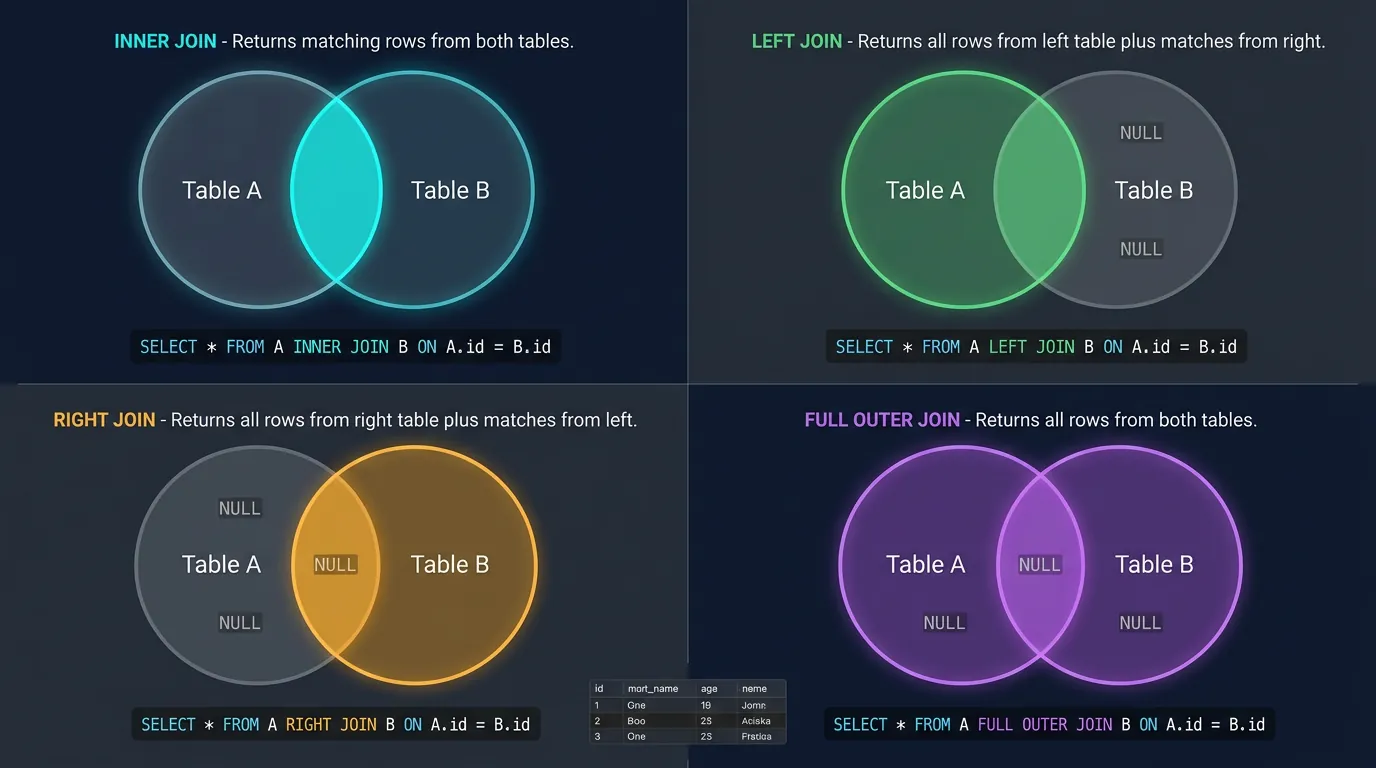
SQL JOIN types visualized as Venn diagrams: INNER, LEFT, RIGHT, and FULL OUTER JOIN
The Phone Book Analogy: Imagine you have two lists: one with names and phone numbers, another with names and addresses. A JOIN matches rows by name, giving you a combined list with names, phones, AND addresses.
Let's set up example tables to demonstrate joins:
-- Example tables for join demonstrations
-- employees table
+----+------------+---------------+
| id | name       | department_id |
+----+------------+---------------+
|  1 | Alice      |             1 |
|  2 | Bob        |             2 |
|  3 | Carol      |             1 |
|  4 | David      |          NULL |  -- No department assigned
+----+------------+---------------+

-- departments table
+----+-------------+
| id | name        |
+----+-------------+
|  1 | Engineering |
|  2 | Marketing   |
|  3 | Sales       |  -- No employees in Sales
+----+-------------+
INNER JOIN
INNER JOIN returns only rows that have matching values in both tables. Non-matching rows are excluded.
-- INNER JOIN: Only employees WITH a department
SELECT
    e.name AS employee_name,
    d.name AS department_name
FROM employees e
INNER JOIN departments d ON e.department_id = d.id;

-- Result:
-- | employee_name | department_name |
-- |---------------|-----------------|
-- | Alice         | Engineering     |
-- | Bob           | Marketing       |
-- | Carol         | Engineering     |
-- David is excluded (NULL department_id)
-- Sales is excluded (no employees)
Visualizing INNER JOIN
Think of two overlapping circles (a Venn diagram). INNER JOIN returns only the intersection—rows that exist in both tables.
LEFT JOIN returns all rows from the left table, plus matching rows from the right table. Non-matching right rows become NULL.
-- LEFT JOIN: ALL employees, even without departments
SELECT
    e.name AS employee_name,
    d.name AS department_name
FROM employees e
LEFT JOIN departments d ON e.department_id = d.id;

-- Result:
-- | employee_name | department_name |
-- |---------------|-----------------|
-- | Alice         | Engineering     |
-- | Bob           | Marketing       |
-- | Carol         | Engineering     |
-- | David         | NULL            |  -- Included, but no matching department

-- RIGHT JOIN: ALL departments, even without employees
SELECT
    e.name AS employee_name,
    d.name AS department_name
FROM employees e
RIGHT JOIN departments d ON e.department_id = d.id;

-- Result:
-- | employee_name | department_name |
-- |---------------|-----------------|
-- | Alice         | Engineering     |
-- | Carol         | Engineering     |
-- | Bob           | Marketing       |
-- | NULL          | Sales           |  -- Included, but no employees
Pro Tip: RIGHT JOIN is rarely used—you can always rewrite it as a LEFT JOIN by swapping table order. Stick with LEFT JOIN for consistency.
FULL OUTER JOIN
FULL OUTER JOIN returns all rows from both tables, matching where possible, with NULLs where there's no match.
-- FULL OUTER JOIN: All employees AND all departments
SELECT
    e.name AS employee_name,
    d.name AS department_name
FROM employees e
FULL OUTER JOIN departments d ON e.department_id = d.id;

-- Result:
-- | employee_name | department_name |
-- |---------------|-----------------|
-- | Alice         | Engineering     |
-- | Bob           | Marketing       |
-- | Carol         | Engineering     |
-- | David         | NULL            |  -- Employee without department
-- | NULL          | Sales           |  -- Department without employees

-- Find unmatched rows (useful for data validation)
SELECT
    e.name AS employee_name,
    d.name AS department_name
FROM employees e
FULL OUTER JOIN departments d ON e.department_id = d.id
WHERE e.id IS NULL OR d.id IS NULL;  -- Only orphaned rows
Join Types Summary
Join Type
Returns
Use Case
INNER JOIN
Only matching rows
Default choice when you only want complete data
LEFT JOIN
All left + matching right
When you need all items from the "main" table
RIGHT JOIN
All right + matching left
Rarely used—rewrite as LEFT JOIN
FULL OUTER
All rows from both
Finding orphaned/unmatched records
CROSS JOIN
Cartesian product (all combinations)
Generating test data, matrix calculations
-- Joining multiple tables (common in real applications)
SELECT
    o.id AS order_id,
    c.name AS customer_name,
    p.name AS product_name,
    oi.quantity,
    oi.unit_price,
    (oi.quantity * oi.unit_price) AS line_total
FROM orders o
INNER JOIN customers c ON o.customer_id = c.id
INNER JOIN order_items oi ON o.id = oi.order_id
INNER JOIN products p ON oi.product_id = p.id
WHERE o.order_date >= '2024-01-01'
ORDER BY o.order_date DESC;
Constraints: Data Integrity Rules
Constraints are rules enforced by the database to ensure data integrity. They prevent bad data from entering your tables—like a bouncer at a club checking IDs.
PRIMARY KEY & FOREIGN KEY
We covered primary keys earlier. Foreign Keys create relationships between tables—they reference the primary key of another table.
-- Creating tables with foreign key relationships
CREATE TABLE departments (
    id SERIAL PRIMARY KEY,
    name VARCHAR(100) NOT NULL,
    budget DECIMAL(15, 2)
);

CREATE TABLE employees (
    id SERIAL PRIMARY KEY,
    first_name VARCHAR(50) NOT NULL,
    last_name VARCHAR(50) NOT NULL,
    email VARCHAR(100) UNIQUE NOT NULL,
    department_id INT,
    hire_date DATE DEFAULT CURRENT_DATE,

    -- Foreign key constraint
    FOREIGN KEY (department_id) REFERENCES departments(id)
        ON DELETE SET NULL     -- If department deleted, set to NULL
        ON UPDATE CASCADE      -- If department id changes, update here too
);

-- Alternative syntax (inline constraint)
CREATE TABLE orders (
    id SERIAL PRIMARY KEY,
    customer_id INT NOT NULL REFERENCES customers(id),
    order_date TIMESTAMP DEFAULT CURRENT_TIMESTAMP,
    total DECIMAL(10, 2) NOT NULL
);
Foreign Key Actions
What happens when the referenced row is deleted or updated?
Action
On DELETE
On UPDATE
CASCADE
Delete child rows too
Update foreign keys
SET NULL
Set foreign key to NULL
Set foreign key to NULL
SET DEFAULT
Set to default value
Set to default value
RESTRICT
Block deletion (error)
Block update (error)
NO ACTION
Same as RESTRICT
Same as RESTRICT
UNIQUE, CHECK, NOT NULL & DEFAULT
-- NOT NULL: Column cannot be empty
CREATE TABLE products (
    id SERIAL PRIMARY KEY,
    name VARCHAR(100) NOT NULL,          -- Required field
    description TEXT,                     -- Optional (NULL allowed)
    price DECIMAL(10, 2) NOT NULL
);

-- UNIQUE: No duplicate values (but allows multiple NULLs)
CREATE TABLE users (
    id SERIAL PRIMARY KEY,
    username VARCHAR(50) UNIQUE NOT NULL,
    email VARCHAR(100) UNIQUE NOT NULL,
    phone VARCHAR(20) UNIQUE             -- Can be NULL, but if set, must be unique
);

-- DEFAULT: Automatic value if none provided
CREATE TABLE orders (
    id SERIAL PRIMARY KEY,
    status VARCHAR(20) DEFAULT 'pending',
    created_at TIMESTAMP DEFAULT CURRENT_TIMESTAMP,
    is_active BOOLEAN DEFAULT true
);

-- CHECK: Custom validation rules
CREATE TABLE employees (
    id SERIAL PRIMARY KEY,
    name VARCHAR(100) NOT NULL,
    age INT CHECK (age >= 18 AND age <= 120),
    salary DECIMAL(10, 2) CHECK (salary > 0),
    email VARCHAR(100) CHECK (email LIKE '%@%.%'),
    start_date DATE CHECK (start_date <= CURRENT_DATE)
);

-- Multiple constraints combined
CREATE TABLE inventory (
    id SERIAL PRIMARY KEY,
    product_id INT NOT NULL REFERENCES products(id),
    warehouse_id INT NOT NULL REFERENCES warehouses(id),
    quantity INT NOT NULL DEFAULT 0 CHECK (quantity >= 0),
    last_updated TIMESTAMP DEFAULT CURRENT_TIMESTAMP,

    -- Composite unique constraint (no duplicate product in same warehouse)
    UNIQUE (product_id, warehouse_id)
);
Constraint Best Practices:
Add constraints during table creation—retrofitting is harder
Use meaningful constraint names for easier debugging
Validate data in application code AND database constraints (defense in depth)
Be careful with CHECK constraints—they can't reference other tables
Views & Stored Queries
A view is a saved query that acts like a virtual table. Think of it as a window into your data that shows exactly what you want to see—no more, no less.
Why use views?
Simplification: Hide complex JOINs behind a simple name
Security: Expose only certain columns to specific users
Consistency: Same business logic used everywhere
Abstraction: Change underlying tables without breaking applications
-- Basic view: Active customers with their order totals
CREATE VIEW active_customer_summary AS
SELECT
    c.id,
    c.first_name || ' ' || c.last_name AS full_name,
    c.email,
    COUNT(o.id) AS total_orders,
    COALESCE(SUM(o.total), 0) AS lifetime_value,
    MAX(o.order_date) AS last_order_date
FROM customers c
LEFT JOIN orders o ON c.id = o.customer_id
WHERE c.is_active = true
GROUP BY c.id, c.first_name, c.last_name, c.email;

-- Using the view (just like a regular table!)
SELECT * FROM active_customer_summary
WHERE lifetime_value > 1000
ORDER BY lifetime_value DESC;

-- View for reporting: Monthly sales summary
CREATE VIEW monthly_sales_report AS
SELECT
    DATE_TRUNC('month', order_date) AS month,
    COUNT(*) AS order_count,
    SUM(total) AS revenue,
    AVG(total) AS avg_order_value,
    COUNT(DISTINCT customer_id) AS unique_customers
FROM orders
WHERE status = 'completed'
GROUP BY DATE_TRUNC('month', order_date);

-- Security view: Hide sensitive columns
CREATE VIEW public_employee_directory AS
SELECT
    id,
    first_name,
    last_name,
    department,
    job_title,
    office_location
    -- Note: salary, SSN, personal_email are NOT included
FROM employees
WHERE employment_status = 'active';
Modifying & Dropping Views
-- Update an existing view (PostgreSQL)
CREATE OR REPLACE VIEW active_customer_summary AS
SELECT
    c.id,
    c.first_name || ' ' || c.last_name AS full_name,
    c.email,
    c.phone,  -- Added new column
    COUNT(o.id) AS total_orders,
    COALESCE(SUM(o.total), 0) AS lifetime_value
FROM customers c
LEFT JOIN orders o ON c.id = o.customer_id
WHERE c.is_active = true
GROUP BY c.id, c.first_name, c.last_name, c.email, c.phone;

-- Rename a view
ALTER VIEW monthly_sales_report RENAME TO sales_monthly_summary;

-- Delete a view
DROP VIEW IF EXISTS old_unused_view;

-- Delete with dependencies check
DROP VIEW active_customer_summary CASCADE;  -- Also drops dependent views
DROP VIEW active_customer_summary RESTRICT; -- Fails if other objects depend on it
Types of Views
View Type
Description
Updatable?
Simple View
Single table, no GROUP BY, no DISTINCT
✅ Yes
Complex View
JOINs, aggregations, subqueries
❌ Usually no
Materialized View
Physically stored, needs refresh
❌ No
Materialized Views (covered in Part 6: Query Optimization) store query results physically—great for slow, complex queries that don't need real-time data.
Performance Note: Views don't store data—they execute their query every time you use them. For frequently-accessed complex views, consider materialized views or indexed views (SQL Server).
SQL Best Practices
Writing SQL that works is easy. Writing SQL that's readable, maintainable, and performant takes practice. Here are professional habits to develop from day one.
Naming Conventions
Consistent Naming Standards
Element
Convention
Good ✅
Bad ❌
Tables
Plural, snake_case
customers, order_items
Customer, tblOrderItem
Columns
Singular, snake_case
first_name, created_at
FirstName, fName
Primary Key
id or table_id
id, customer_id
CustomerID, pk_id
Foreign Key
referenced_table_id
customer_id, order_id
custID, fk_customer
Boolean
is_ or has_ prefix
is_active, has_paid
active, paid_flag
Timestamps
_at suffix
created_at, updated_at
creation_date, modified
Code Formatting & Style
-- ❌ BAD: Hard to read
SELECT c.id,c.first_name,c.last_name,o.order_date,o.total FROM customers c JOIN orders o ON c.id=o.customer_id WHERE o.total>100 AND c.is_active=true ORDER BY o.order_date DESC;

-- ✅ GOOD: Well-formatted and readable
SELECT
    c.id,
    c.first_name,
    c.last_name,
    o.order_date,
    o.total
FROM customers c
INNER JOIN orders o ON c.id = o.customer_id
WHERE o.total > 100
    AND c.is_active = true
ORDER BY o.order_date DESC;
Formatting Rules:
Use UPPERCASE for SQL keywords (SELECT, FROM, WHERE, etc.)
Put each major clause on its own line
Indent continuation lines (AND, OR conditions)
Add spaces around operators (=, >, <, +, -, etc.)
Use meaningful table aliases (c for customers, not x or t1)
Comment complex logic and business rules
Performance Tips
-- ❌ BAD: SELECT * fetches unnecessary data
SELECT * FROM customers;

-- ✅ GOOD: Only select columns you need
SELECT id, first_name, email FROM customers;

-- ❌ BAD: Using functions on indexed columns prevents index usage
SELECT * FROM orders WHERE YEAR(order_date) = 2024;

-- ✅ GOOD: Let the index work for you
SELECT * FROM orders
WHERE order_date >= '2024-01-01'
  AND order_date < '2025-01-01';

-- ❌ BAD: Leading wildcards prevent index usage
SELECT * FROM products WHERE name LIKE '%widget%';

-- ✅ BETTER: Trailing wildcard can use index
SELECT * FROM products WHERE name LIKE 'widget%';

-- ❌ BAD: N+1 query pattern (in application code loops)
-- For each order, run a separate query for customer

-- ✅ GOOD: Single query with JOIN
SELECT o.*, c.first_name, c.last_name
FROM orders o
JOIN customers c ON o.customer_id = c.id
WHERE o.status = 'pending';
Security Practices
NEVER Concatenate User Input Into SQL!
-- ❌ DANGEROUS: SQL Injection vulnerability!
-- query = "SELECT * FROM users WHERE username = '" + user_input + "'"
-- If user_input = "admin'; DROP TABLE users; --", disaster strikes!

-- ✅ SAFE: Use parameterized queries (example in Python)
-- cursor.execute("SELECT * FROM users WHERE username = %s", (user_input,))

-- ✅ SAFE: Use prepared statements (example in PostgreSQL)
PREPARE get_user (text) AS
    SELECT * FROM users WHERE username = $1;
EXECUTE get_user('john_doe');
Pre-Production Query Checklist
Before Running in Production
Ask yourself these questions before executing any query on production data:
☐ UPDATE/DELETE: Did I include a WHERE clause?
☐ WHERE clause: Does it target the right rows? Test with SELECT first!
☐ Backup: Do I have a recent backup if things go wrong?
☐ Transaction: Should I wrap this in BEGIN/ROLLBACK for safety?
☐ Performance: Have I checked EXPLAIN for large tables?
☐ Off-hours: Should this run during low-traffic periods?
☐ Logging: Am I tracking what I'm changing for audit purposes?
Conclusion & Next Steps
You've now mastered the fundamentals of SQL—the foundation upon which all database work is built. From basic CRUD operations to complex joins and constraints, these skills form the core of database interaction.
Continue the Database Mastery Series
Part 2: Advanced SQL & Query Mastery
Master CTEs, window functions, stored procedures, and advanced query techniques.