Introduction to Sequential Models
Recurrent neural networks process sequences by maintaining hidden states that capture information from previous time steps. This enables modeling of temporal dependencies in language.
Key Insight
RNNs, LSTMs, and GRUs share information across time steps through hidden states, with LSTMs and GRUs using gating mechanisms to control information flow and mitigate vanishing gradients.
NLP Mastery
NLP Fundamentals & Linguistic Basics
Phonology, morphology, syntax, semantics, pragmaticsTokenization & Text Cleaning
Subword tokenization, BPE, stopwords, normalizationText Representation & Feature Engineering
Bag-of-words, TF-IDF, feature extraction, vectorizationWord Embeddings
Word2Vec, GloVe, FastText, embedding spaces, analogiesStatistical Language Models & N-grams
Probability chains, smoothing, perplexity, Markov modelsNeural Networks for NLP
Feedforward nets, backpropagation, activation functionsRNNs, LSTMs & GRUs
Sequence modeling, vanishing gradients, gated architecturesTransformers & Attention Mechanism
Self-attention, multi-head attention, positional encodingPretrained Language Models & Transfer Learning
BERT, RoBERTa, fine-tuning, feature extractionGPT Models & Text Generation
Autoregressive generation, prompting, GPT architectureCore NLP Tasks
NER, POS tagging, sentiment analysis, text classificationAdvanced NLP Tasks
Question answering, summarization, machine translationMultilingual & Cross-lingual NLP
mBERT, XLM-R, zero-shot transfer, language diversityEvaluation, Ethics & Responsible NLP
BLEU, ROUGE, bias detection, fairness, responsible AINLP Systems, Optimization & Production
Model serving, quantization, distillation, deploymentCutting-Edge & Research Topics
LLMs, multimodal NLP, reasoning, emerging researchVanilla RNNs
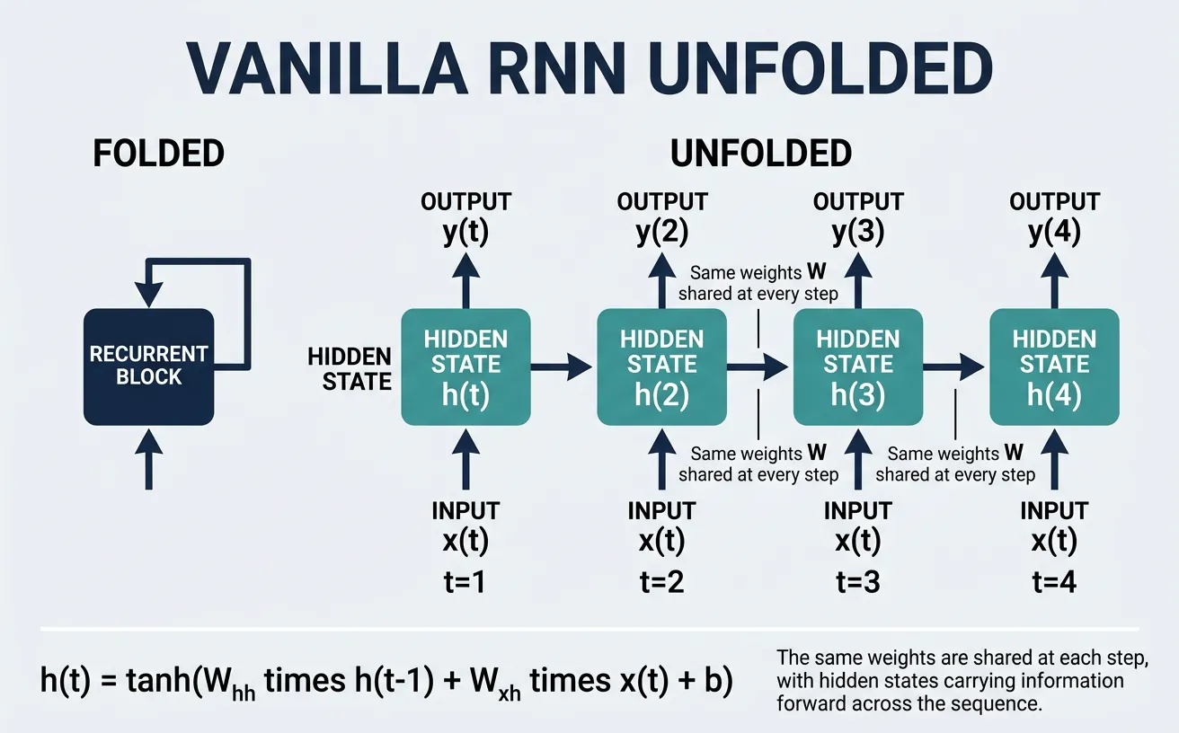
Recurrent Neural Networks (RNNs) are a class of neural networks designed specifically for processing sequential data. Unlike feedforward networks that treat each input independently, RNNs maintain a hidden state that captures information from previous time steps, allowing them to model temporal dependencies in data. This makes them particularly well-suited for natural language processing tasks where the meaning of a word often depends on the words that came before it.
The fundamental insight behind RNNs is weight sharing across time steps. The same set of weights is applied at each position in the sequence, which means the network learns patterns that can occur at any position. This is similar to how convolutional networks share weights across spatial positions, enabling the model to recognize patterns regardless of their location in the input.
Architecture
The vanilla RNN processes a sequence one element at a time, maintaining a hidden state vector that acts as the network's "memory." At each time step $t$, the RNN takes two inputs: the current input $x_t$ and the previous hidden state $h_{t-1}$. It produces a new hidden state $h_t$ and optionally an output $y_t$. The mathematical formulation is elegantly simple: the hidden state is computed by applying a non-linear activation function (typically $\tanh$) to a linear combination of the input and previous hidden state.
RNN Architecture Diagram
flowchart LR
    x0["x₀"] --> c0["RNN Cell"]
    x1["x₁"] --> c1["RNN Cell"]
    x2["x₂"] --> c2["RNN Cell"]
    x3["x₃"] --> c3["RNN Cell"]
    c0 -->|"h₀"| c1
    c1 -->|"h₁"| c2
    c2 -->|"h₂"| c3
    c0 --> y0["y₀"]
    c1 --> y1["y₁"]
    c2 --> y2["y₂"]
    c3 --> y3["y₃"]
Hidden State Update:
$$h_t = \tanh(W_{xh} \cdot x_t + W_{hh} \cdot h_{t-1} + b_h)$$
Output Computation:
$$y_t = W_{hy} \cdot h_t + b_y$$
The key components of an RNN cell are the weight matrices: $W_{xh}$ transforms the input, $W_{hh}$ transforms the previous hidden state, and $W_{hy}$ (if outputs are produced at each step) projects the hidden state to the output space. The hidden state dimension is a hyperparameter that determines the network's capacity to store information.
import torch
import torch.nn as nn

# Basic RNN Cell from scratch
class VanillaRNNCell(nn.Module):
    """Manual implementation of a vanilla RNN cell."""

    def __init__(self, input_size, hidden_size):
        super().__init__()
        self.hidden_size = hidden_size

        # Weight matrices
        self.W_xh = nn.Linear(input_size, hidden_size, bias=False)  # Input to hidden
        self.W_hh = nn.Linear(hidden_size, hidden_size, bias=True)  # Hidden to hidden

    def forward(self, x_t, h_prev):
        """
        Forward pass for single time step.

        Args:
            x_t: Input at time t, shape (batch_size, input_size)
            h_prev: Hidden state from time t-1, shape (batch_size, hidden_size)

        Returns:
            h_t: New hidden state, shape (batch_size, hidden_size)
        """
        # Compute new hidden state
        h_t = torch.tanh(self.W_xh(x_t) + self.W_hh(h_prev))
        return h_t

# Example usage
batch_size = 4
seq_length = 10
input_size = 32
hidden_size = 64

# Create cell and sample input
cell = VanillaRNNCell(input_size, hidden_size)
x = torch.randn(batch_size, seq_length, input_size)  # Input sequence
h = torch.zeros(batch_size, hidden_size)  # Initial hidden state

# Process sequence step by step
outputs = []
for t in range(seq_length):
    h = cell(x[:, t, :], h)
    outputs.append(h)

# Stack outputs: (batch_size, seq_length, hidden_size)
output_sequence = torch.stack(outputs, dim=1)
print(f"Input shape: {x.shape}")
print(f"Output sequence shape: {output_sequence.shape}")
print(f"Final hidden state shape: {h.shape}")
Understanding Hidden State Dimensions
The hidden state dimension controls the network's memory capacity. A larger hidden size allows the RNN to store more information about the sequence history but increases computational cost and the risk of overfitting. Common values range from 64 to 512 for small tasks, and 512 to 2048 for large-scale language modeling. The hidden state can be thought of as a compressed representation of everything the network has seen so far.
import torch
import torch.nn as nn

# Using PyTorch's built-in RNN
class SimpleRNN(nn.Module):
    """RNN for sequence processing using PyTorch nn.RNN."""

    def __init__(self, vocab_size, embedding_dim, hidden_size, output_size):
        super().__init__()
        self.embedding = nn.Embedding(vocab_size, embedding_dim)
        self.rnn = nn.RNN(
            input_size=embedding_dim,
            hidden_size=hidden_size,
            num_layers=1,
            batch_first=True,  # Input: (batch, seq, features)
            nonlinearity='tanh'
        )
        self.fc = nn.Linear(hidden_size, output_size)

    def forward(self, x, h_0=None):
        """
        Args:
            x: Token indices, shape (batch_size, seq_length)
            h_0: Initial hidden state (optional)

        Returns:
            output: Predictions at each time step
            h_n: Final hidden state
        """
        # Embed tokens
        embedded = self.embedding(x)  # (batch, seq, embed_dim)

        # Process through RNN
        # output: hidden states at all time steps
        # h_n: hidden state at final time step
        output, h_n = self.rnn(embedded, h_0)

        # Project to output space
        predictions = self.fc(output)  # (batch, seq, output_size)

        return predictions, h_n

# Example: Language modeling setup
vocab_size = 10000
embedding_dim = 128
hidden_size = 256
output_size = vocab_size  # Predict next token

model = SimpleRNN(vocab_size, embedding_dim, hidden_size, output_size)

# Sample input: batch of 4 sequences, each length 20
x = torch.randint(0, vocab_size, (4, 20))
predictions, final_hidden = model(x)

print(f"Input shape: {x.shape}")
print(f"Predictions shape: {predictions.shape}")
print(f"Final hidden shape: {final_hidden.shape}")
Backpropagation Through Time
Backpropagation Through Time (BPTT) is the algorithm used to train RNNs by computing gradients across time steps. The process involves unrolling the RNN through all time steps, computing the loss, and then backpropagating gradients from the final time step back to the initial one. This effectively treats the unrolled RNN as a very deep feedforward network where each layer corresponds to a time step.
The challenge with BPTT is that for long sequences, we need to store all intermediate hidden states to compute gradients, leading to high memory consumption. Additionally, gradients must flow through many time steps, which creates numerical instability issues. To address memory concerns, Truncated BPTT is often used, where gradients are only backpropagated through a fixed number of time steps rather than the entire sequence.
BPTT Gradient Flow
Forward Pass (left → right):
$$h_0 \to h_1 \to h_2 \to \cdots \to h_T \to \mathcal{L}$$
Backward Pass — right ← left (BPTT):
$$\frac{\partial \mathcal{L}}{\partial h_0} \leftarrow \cdots \leftarrow \frac{\partial \mathcal{L}}{\partial h_T} \leftarrow \mathcal{L}$$
Gradient accumulation for Whh:
$$\frac{\partial \mathcal{L}}{\partial W_{hh}} = \sum_{t=1}^{T} \frac{\partial \mathcal{L}}{\partial h_t} \cdot \frac{\partial h_t}{\partial W_{hh}}$$
Gradient at each time step t:
$$\frac{\partial \mathcal{L}}{\partial h_t} = \frac{\partial \mathcal{L}}{\partial y_t} \cdot \frac{\partial y_t}{\partial h_t} + \frac{\partial \mathcal{L}}{\partial h_{t+1}} \cdot \frac{\partial h_{t+1}}{\partial h_t}$$
import torch
import torch.nn as nn
import torch.optim as optim

# SimpleRNN included here for a self-contained, runnable example
class SimpleRNN(nn.Module):
    """RNN for sequence processing using PyTorch nn.RNN."""

    def __init__(self, vocab_size, embedding_dim, hidden_size, output_size):
        super().__init__()
        self.embedding = nn.Embedding(vocab_size, embedding_dim)
        self.rnn = nn.RNN(
            input_size=embedding_dim,
            hidden_size=hidden_size,
            num_layers=1,
            batch_first=True,
            nonlinearity='tanh'
        )
        self.fc = nn.Linear(hidden_size, output_size)

    def forward(self, x, h_0=None):
        embedded = self.embedding(x)
        output, h_n = self.rnn(embedded, h_0)
        return self.fc(output), h_n

# Demonstrating BPTT with truncated backpropagation
class TruncatedBPTTTrainer:
    """Trainer implementing truncated BPTT for memory efficiency."""

    def __init__(self, model, learning_rate=0.001, bptt_steps=35):
        self.model = model
        self.bptt_steps = bptt_steps
        self.optimizer = optim.Adam(model.parameters(), lr=learning_rate)
        self.criterion = nn.CrossEntropyLoss()

    def train_step(self, sequence, targets):
        """
        Train on a sequence using truncated BPTT.

        Args:
            sequence: Full input sequence (batch, total_length)
            targets: Target tokens (batch, total_length)
        """
        total_loss = 0.0
        num_chunks = 0

        # Initialize hidden state
        hidden = None

        # Process sequence in chunks
        for i in range(0, sequence.size(1) - 1, self.bptt_steps):
            # Get chunk
            chunk_end = min(i + self.bptt_steps, sequence.size(1) - 1)
            x_chunk = sequence[:, i:chunk_end]
            y_chunk = targets[:, i:chunk_end]

            # Detach hidden state to truncate gradient flow
            # This prevents gradients from flowing into previous chunks
            if hidden is not None:
                hidden = hidden.detach()

            # Forward pass
            self.optimizer.zero_grad()
            output, hidden = self.model(x_chunk, hidden)

            # Compute loss (reshape for CrossEntropyLoss)
            loss = self.criterion(
                output.reshape(-1, output.size(-1)),
                y_chunk.reshape(-1)
            )

            # Backward pass (only through this chunk due to detach)
            loss.backward()

            # Gradient clipping to prevent exploding gradients
            torch.nn.utils.clip_grad_norm_(self.model.parameters(), max_norm=5.0)

            # Update parameters
            self.optimizer.step()

            total_loss += loss.item()
            num_chunks += 1

        return total_loss / num_chunks

# Example usage
vocab_size = 5000
model = SimpleRNN(vocab_size, embedding_dim=128, hidden_size=256, output_size=vocab_size)
trainer = TruncatedBPTTTrainer(model, bptt_steps=35)

# Simulate training on a long sequence
long_sequence = torch.randint(0, vocab_size, (2, 200))  # 2 sequences, length 200
targets = torch.randint(0, vocab_size, (2, 200))

avg_loss = trainer.train_step(long_sequence, targets)
print(f"Average loss per chunk: {avg_loss:.4f}")
Vanishing Gradient Problem
The vanishing gradient problem is the fundamental limitation of vanilla RNNs that prevents them from learning long-range dependencies. During backpropagation through time, gradients are multiplied by the weight matrix $W_{hh}$ at each time step. If the largest eigenvalue of $W_{hh}$ is less than 1, gradients decay exponentially as they flow backward; if greater than 1, they explode exponentially. For sequences of length $T$, gradients can shrink by a factor of $\lambda^T$ where $\lambda$ is the dominant eigenvalue.
Consider trying to learn that a word at position 0 is important for predicting a word at position 100. The gradient signal from position 100 must pass through 100 matrix multiplications to reach position 0. With typical weight initializations, this gradient becomes vanishingly small, making it nearly impossible for the network to learn such long-range dependencies. This is why vanilla RNNs typically can only effectively model dependencies spanning 10-20 time steps.
Why Gradients Vanish
Mathematical explanation: When backpropagating through time, we compute $\partial h_T / \partial h_0 = \prod_{t=1}^{T} \partial h_t / \partial h_{t-1}$. Each term involves $W_{hh}$ and the derivative of $\tanh$ (bounded by 1). With $\tanh$ saturation and $\|W_{hh}\| < 1$, this product approaches zero exponentially. The key insight is that gradients decay/explode at a rate determined by the spectral radius of $W_{hh}$ times the average derivative of the activation function.
import torch
import torch.nn as nn
import matplotlib.pyplot as plt
import numpy as np

def analyze_gradient_flow(sequence_length=100, hidden_size=64):
    """
    Visualize how gradients decay in vanilla RNNs.
    """
    # Create a simple RNN
    rnn = nn.RNN(input_size=32, hidden_size=hidden_size, batch_first=True)

    # Input sequence
    x = torch.randn(1, sequence_length, 32, requires_grad=True)
    h0 = torch.zeros(1, 1, hidden_size)

    # Forward pass - get all hidden states
    output, _ = rnn(x, h0)

    # Compute gradients w.r.t. final hidden state
    # We want to see how much the final output depends on each time step
    final_output = output[0, -1, :].sum()  # Scalar loss from final state
    final_output.backward()

    # Examine gradient magnitudes at each time step
    # x.grad shows how much each input position affects the final output
    grad_norms = []
    for t in range(sequence_length):
        grad_norm = x.grad[0, t, :].norm().item()
        grad_norms.append(grad_norm)

    # Plot gradient flow
    plt.figure(figsize=(12, 5))

    plt.subplot(1, 2, 1)
    plt.plot(range(sequence_length), grad_norms)
    plt.xlabel('Time Step')
    plt.ylabel('Gradient Norm')
    plt.title('Gradient Magnitude vs. Time Step (Vanilla RNN)')
    plt.yscale('log')  # Log scale to see exponential decay

    plt.subplot(1, 2, 2)
    plt.plot(range(sequence_length), grad_norms)
    plt.xlabel('Time Step')
    plt.ylabel('Gradient Norm')
    plt.title('Linear Scale View')

    plt.tight_layout()
    plt.savefig('gradient_flow.png', dpi=150, bbox_inches='tight')
    plt.show()

    print(f"Gradient at t=0: {grad_norms[0]:.6f}")
    print(f"Gradient at t={sequence_length//2}: {grad_norms[sequence_length//2]:.6f}")
    print(f"Gradient at t={sequence_length-1}: {grad_norms[-1]:.6f}")
    print(f"Decay ratio (t=0 vs t={sequence_length-1}): {grad_norms[0]/grad_norms[-1]:.2f}x")

# Run analysis
analyze_gradient_flow(sequence_length=100, hidden_size=64)
import torch
import torch.nn as nn

def demonstrate_vanishing_exploding_gradients():
    """
    Show the effect of weight initialization on gradient flow.
    """
    hidden_size = 100
    sequence_length = 50

    # Case 1: Weights initialized to cause vanishing gradients
    print("=== Vanishing Gradient Scenario ===")
    W_small = torch.randn(hidden_size, hidden_size) * 0.1  # Small weights
    eigenvalues = torch.linalg.eigvals(W_small)
    spectral_radius = eigenvalues.abs().max().item()
    print(f"Spectral radius: {spectral_radius:.4f}")

    # Simulate gradient flow
    gradient = torch.ones(hidden_size)
    for t in range(sequence_length):
        gradient = torch.tanh(W_small @ gradient) * 0.5  # tanh derivative ~ 0.5 on average
    print(f"Gradient norm after {sequence_length} steps: {gradient.norm():.10f}")

    # Case 2: Weights initialized to cause exploding gradients
    print("\n=== Exploding Gradient Scenario ===")
    W_large = torch.randn(hidden_size, hidden_size) * 1.5  # Large weights
    eigenvalues = torch.linalg.eigvals(W_large)
    spectral_radius = eigenvalues.abs().max().item()
    print(f"Spectral radius: {spectral_radius:.4f}")

    gradient = torch.ones(hidden_size)
    for t in range(sequence_length):
        gradient = W_large @ gradient  # Ignoring activation for demonstration
        if gradient.norm() > 1e10:
            print(f"Gradient exploded at step {t}!")
            break
    print(f"Gradient norm: {gradient.norm():.2e}")

    # Case 3: Orthogonal initialization (helps but doesn't fully solve)
    print("\n=== Orthogonal Initialization ===")
    W_ortho = nn.init.orthogonal_(torch.empty(hidden_size, hidden_size))
    eigenvalues = torch.linalg.eigvals(W_ortho)
    spectral_radius = eigenvalues.abs().max().item()
    print(f"Spectral radius: {spectral_radius:.4f}")

    gradient = torch.ones(hidden_size)
    for t in range(sequence_length):
        # Even with orthogonal weights, tanh still causes vanishing
        gradient = torch.tanh(W_ortho @ gradient)
    print(f"Gradient norm after {sequence_length} steps: {gradient.norm():.6f}")

demonstrate_vanishing_exploding_gradients()
Long Short-Term Memory (LSTM)
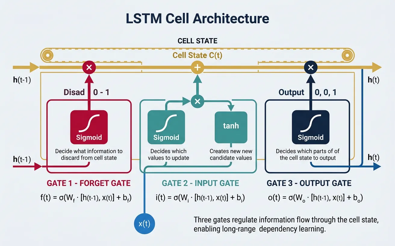
Long Short-Term Memory (LSTM) networks were introduced by Hochreiter and Schmidhuber in 1997 specifically to address the vanishing gradient problem. The key innovation is the cell state, a separate pathway that allows information to flow across many time steps with minimal modification. Think of the cell state as a conveyor belt running through the entire sequence—information can be added or removed via carefully regulated gates, but the default behavior is to pass information unchanged.
LSTMs introduce three gating mechanisms that control information flow: the forget gate decides what information to discard from the cell state, the input gate determines what new information to store, and the output gate controls what parts of the cell state to output as the hidden state. Each gate is a neural network layer with sigmoid activation, producing values between 0 (completely block) and 1 (completely pass through).
Gates & Cell State
LSTM Gate Architecture
flowchart TD
    IN["Input: h_prev, x_t"] --> FG["Forget Gate f_t"]
    IN --> IG["Input Gate i_t"]
    IN --> CC["Candidate C_tilde"]
    IN --> OG["Output Gate o_t"]
    CP["Cell State C_prev"] --> CT["Cell State C_t"]
    FG --> CT
    IG --> CT
    CC --> CT
    CT --> HT["Hidden State h_t"]
    OG --> HT
Gate Equations:
$$f_t = \sigma(W_f \cdot [h_{t-1}, x_t] + b_f) \quad \text{(forget gate)}$$
$$i_t = \sigma(W_i \cdot [h_{t-1}, x_t] + b_i) \quad \text{(input gate)}$$
$$\tilde{C}_t = \tanh(W_C \cdot [h_{t-1}, x_t] + b_C) \quad \text{(candidate)}$$
$$C_t = f_t \odot C_{t-1} + i_t \odot \tilde{C}_t \quad \text{(new cell state)}$$
$$o_t = \sigma(W_o \cdot [h_{t-1}, x_t] + b_o) \quad \text{(output gate)}$$
$$h_t = o_t \odot \tanh(C_t) \quad \text{(hidden state)}$$
Key insight: Cell state enables direct gradient flow — $\partial C_t / \partial C_{t-1} = f_t$ (no weight multiplication, values 0–1).
import torch
import torch.nn as nn

class LSTMCellManual(nn.Module):
    """
    Manual implementation of LSTM cell to understand gate mechanics.
    """

    def __init__(self, input_size, hidden_size):
        super().__init__()
        self.hidden_size = hidden_size

        # Combined weight matrix for efficiency (all 4 gates together)
        # Order: input gate, forget gate, cell gate, output gate
        self.gates = nn.Linear(input_size + hidden_size, 4 * hidden_size)

        # Initialize forget gate bias to 1.0 (important for training stability)
        # This encourages the network to remember by default
        nn.init.constant_(self.gates.bias[hidden_size:2*hidden_size], 1.0)

    def forward(self, x_t, states):
        """
        Forward pass for single time step.

        Args:
            x_t: Input at time t, shape (batch_size, input_size)
            states: Tuple of (h_{t-1}, C_{t-1}), each (batch_size, hidden_size)

        Returns:
            h_t: New hidden state
            c_t: New cell state
        """
        h_prev, c_prev = states

        # Concatenate input and previous hidden state
        combined = torch.cat([x_t, h_prev], dim=1)

        # Compute all gates in one operation
        gates = self.gates(combined)

        # Split into individual gates
        i_gate, f_gate, c_tilde, o_gate = gates.chunk(4, dim=1)

        # Apply activations
        i_gate = torch.sigmoid(i_gate)      # Input gate
        f_gate = torch.sigmoid(f_gate)      # Forget gate
        c_tilde = torch.tanh(c_tilde)       # Candidate cell state
        o_gate = torch.sigmoid(o_gate)      # Output gate

        # Update cell state: forget old info + add new info
        c_t = f_gate * c_prev + i_gate * c_tilde

        # Compute hidden state
        h_t = o_gate * torch.tanh(c_t)

        return h_t, c_t

# Example usage
batch_size = 4
input_size = 32
hidden_size = 64

cell = LSTMCellManual(input_size, hidden_size)

# Initial states
h = torch.zeros(batch_size, hidden_size)
c = torch.zeros(batch_size, hidden_size)

# Single input
x = torch.randn(batch_size, input_size)

# Forward pass
h_new, c_new = cell(x, (h, c))

print(f"Input shape: {x.shape}")
print(f"Hidden state shape: {h_new.shape}")
print(f"Cell state shape: {c_new.shape}")
Why LSTMs Solve Vanishing Gradients
The cell state provides an "information highway." When computing $\partial C_t / \partial C_{t-1}$, we get $f_t$ (the forget gate value), which is a scalar between 0 and 1—not a weight matrix multiplication. If the forget gate is close to 1 (remember), gradients flow directly backward with minimal decay. The network learns when to let gradients pass (large $f_t$) and when to gate them (small $f_t$). This is fundamentally different from vanilla RNNs where gradients always pass through $W_{hh}$.
import torch
import torch.nn as nn

# Complete LSTM for sequence processing
class LSTMLanguageModel(nn.Module):
    """
    LSTM-based language model for next token prediction.
    """

    def __init__(self, vocab_size, embedding_dim, hidden_size, num_layers=2, dropout=0.3):
        super().__init__()

        self.embedding = nn.Embedding(vocab_size, embedding_dim)
        self.dropout = nn.Dropout(dropout)

        self.lstm = nn.LSTM(
            input_size=embedding_dim,
            hidden_size=hidden_size,
            num_layers=num_layers,
            batch_first=True,
            dropout=dropout if num_layers > 1 else 0,  # Dropout between layers
        )

        self.fc = nn.Linear(hidden_size, vocab_size)

        # Tie embedding and output weights (optional, reduces parameters)
        if embedding_dim == hidden_size:
            self.fc.weight = self.embedding.weight

    def forward(self, x, hidden=None):
        """
        Args:
            x: Token indices (batch_size, seq_length)
            hidden: Optional tuple (h_0, c_0) for initial states

        Returns:
            logits: Predictions (batch_size, seq_length, vocab_size)
            hidden: Final (h_n, c_n) states
        """
        # Embed and apply dropout
        embedded = self.dropout(self.embedding(x))

        # LSTM forward pass
        # output: all hidden states (batch, seq, hidden_size)
        # hidden: tuple of (h_n, c_n), each (num_layers, batch, hidden_size)
        output, hidden = self.lstm(embedded, hidden)

        # Apply dropout and project to vocabulary
        output = self.dropout(output)
        logits = self.fc(output)

        return logits, hidden

    def init_hidden(self, batch_size, device):
        """Initialize hidden states to zeros."""
        num_layers = self.lstm.num_layers
        hidden_size = self.lstm.hidden_size

        h_0 = torch.zeros(num_layers, batch_size, hidden_size, device=device)
        c_0 = torch.zeros(num_layers, batch_size, hidden_size, device=device)

        return (h_0, c_0)

# Example usage
vocab_size = 10000
embedding_dim = 256
hidden_size = 256
num_layers = 2

model = LSTMLanguageModel(vocab_size, embedding_dim, hidden_size, num_layers)

# Sample input
batch_size = 4
seq_length = 50
x = torch.randint(0, vocab_size, (batch_size, seq_length))

# Initialize hidden state
hidden = model.init_hidden(batch_size, x.device)

# Forward pass
logits, hidden = model(x, hidden)

print(f"Input: {x.shape}")
print(f"Output logits: {logits.shape}")
print(f"Hidden h_n: {hidden[0].shape}")
print(f"Hidden c_n: {hidden[1].shape}")
LSTM Variants
Several LSTM variants have been proposed to improve performance or reduce computational cost. Peephole connections allow gates to look at the cell state directly, not just the hidden state. The Coupled Input-Forget Gate (CIFG) ties the input and forget gates together as $i_t = 1 - f_t$, reducing parameters. Multiplicative LSTM uses the hidden state to modulate the weight matrix rather than just adding it.
import torch
import torch.nn as nn

class PeepholeLSTMCell(nn.Module):
    """
    LSTM with peephole connections.
    Gates can see the cell state directly.
    """

    def __init__(self, input_size, hidden_size):
        super().__init__()
        self.hidden_size = hidden_size

        # Standard gates (input + hidden)
        self.W_i = nn.Linear(input_size + hidden_size, hidden_size)
        self.W_f = nn.Linear(input_size + hidden_size, hidden_size)
        self.W_c = nn.Linear(input_size + hidden_size, hidden_size)
        self.W_o = nn.Linear(input_size + hidden_size, hidden_size)

        # Peephole weights (diagonal, so just vectors)
        self.p_i = nn.Parameter(torch.randn(hidden_size))  # Input gate peephole
        self.p_f = nn.Parameter(torch.randn(hidden_size))  # Forget gate peephole
        self.p_o = nn.Parameter(torch.randn(hidden_size))  # Output gate peephole

    def forward(self, x_t, states):
        h_prev, c_prev = states
        combined = torch.cat([x_t, h_prev], dim=1)

        # Gates with peephole connections to cell state
        i_gate = torch.sigmoid(self.W_i(combined) + self.p_i * c_prev)
        f_gate = torch.sigmoid(self.W_f(combined) + self.p_f * c_prev)
        c_tilde = torch.tanh(self.W_c(combined))

        c_t = f_gate * c_prev + i_gate * c_tilde

        # Output gate uses new cell state
        o_gate = torch.sigmoid(self.W_o(combined) + self.p_o * c_t)
        h_t = o_gate * torch.tanh(c_t)

        return h_t, c_t


class CoupledLSTMCell(nn.Module):
    """
    LSTM with Coupled Input-Forget Gate (CIFG).
    i_t = 1 - f_t, reducing parameters.
    """

    def __init__(self, input_size, hidden_size):
        super().__init__()
        self.hidden_size = hidden_size

        # Only need forget gate (input gate is derived)
        self.W_f = nn.Linear(input_size + hidden_size, hidden_size)
        self.W_c = nn.Linear(input_size + hidden_size, hidden_size)
        self.W_o = nn.Linear(input_size + hidden_size, hidden_size)

        # Initialize forget gate bias to 1.0
        nn.init.constant_(self.W_f.bias, 1.0)

    def forward(self, x_t, states):
        h_prev, c_prev = states
        combined = torch.cat([x_t, h_prev], dim=1)

        # Only compute forget gate; input gate is complement
        f_gate = torch.sigmoid(self.W_f(combined))
        i_gate = 1.0 - f_gate  # Coupled!

        c_tilde = torch.tanh(self.W_c(combined))
        c_t = f_gate * c_prev + i_gate * c_tilde

        o_gate = torch.sigmoid(self.W_o(combined))
        h_t = o_gate * torch.tanh(c_t)

        return h_t, c_t


# Compare parameter counts
input_size, hidden_size = 128, 256

standard_params = sum(p.numel() for p in LSTMCellManual(input_size, hidden_size).parameters())
peephole_params = sum(p.numel() for p in PeepholeLSTMCell(input_size, hidden_size).parameters())
coupled_params = sum(p.numel() for p in CoupledLSTMCell(input_size, hidden_size).parameters())

print(f"Standard LSTM parameters: {standard_params:,}")
print(f"Peephole LSTM parameters: {peephole_params:,}")
print(f"Coupled LSTM parameters: {coupled_params:,}")
print(f"Coupled saves {standard_params - coupled_params:,} parameters ({100*(1-coupled_params/standard_params):.1f}%)")
Gated Recurrent Units (GRU)
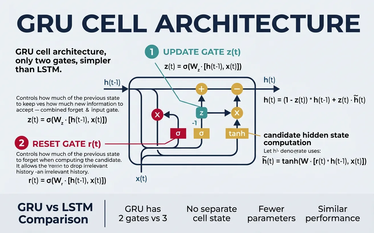
Gated Recurrent Units (GRUs), introduced by Cho et al. in 2014, offer a simpler alternative to LSTMs while maintaining similar performance on many tasks. GRUs combine the forget and input gates into a single update gate and merge the cell state and hidden state into one. This results in fewer parameters and faster training, making GRUs popular for tasks where computational efficiency is important.
The GRU uses two gates: the reset gate determines how much of the previous hidden state to ignore when computing the candidate hidden state, and the update gate controls the balance between the old hidden state and the new candidate. When the update gate is 0, the hidden state is completely replaced; when it's 1, the old state is kept unchanged. This design captures the essential gating mechanisms of LSTMs with less complexity.
GRU Architecture
flowchart TD
    IN["Input: h_prev, x_t"] --> UG["Update Gate z_t"]
    IN --> RG["Reset Gate r_t"]
    RG -->|"r_t × h_prev"| CH["Candidate h_tilde"]
    UG --> NH["New Hidden h_t"]
    CH --> NH
Gate Equations:
$$z_t = \sigma(W_z \cdot [h_{t-1}, x_t]) \quad \text{(update gate)}$$
$$r_t = \sigma(W_r \cdot [h_{t-1}, x_t]) \quad \text{(reset gate)}$$
$$\tilde{h}_t = \tanh(W \cdot [r_t \odot h_{t-1}, x_t]) \quad \text{(candidate)}$$
$$h_t = (1 - z_t) \odot h_{t-1} + z_t \odot \tilde{h}_t \quad \text{(new hidden state)}$$
import torch
import torch.nn as nn

class GRUCellManual(nn.Module):
    """
    Manual implementation of GRU cell.
    """

    def __init__(self, input_size, hidden_size):
        super().__init__()
        self.hidden_size = hidden_size

        # Update gate
        self.W_z = nn.Linear(input_size + hidden_size, hidden_size)
        # Reset gate
        self.W_r = nn.Linear(input_size + hidden_size, hidden_size)
        # Candidate hidden state
        self.W_h = nn.Linear(input_size + hidden_size, hidden_size)

    def forward(self, x_t, h_prev):
        """
        Args:
            x_t: Input (batch_size, input_size)
            h_prev: Previous hidden state (batch_size, hidden_size)

        Returns:
            h_t: New hidden state
        """
        combined = torch.cat([h_prev, x_t], dim=1)

        # Compute gates
        z_t = torch.sigmoid(self.W_z(combined))  # Update gate
        r_t = torch.sigmoid(self.W_r(combined))  # Reset gate

        # Candidate hidden state (reset gate applied to h_prev)
        combined_reset = torch.cat([r_t * h_prev, x_t], dim=1)
        h_tilde = torch.tanh(self.W_h(combined_reset))

        # Interpolate between old and new
        h_t = (1 - z_t) * h_prev + z_t * h_tilde

        return h_t

# Example
batch_size = 4
input_size = 32
hidden_size = 64

gru_cell = GRUCellManual(input_size, hidden_size)
h = torch.zeros(batch_size, hidden_size)
x = torch.randn(batch_size, input_size)

h_new = gru_cell(x, h)
print(f"GRU output shape: {h_new.shape}")
LSTM vs GRU: When to Use Each
Choose GRU when: You need faster training, have limited data, or computational resources are constrained. GRUs have ~25% fewer parameters than LSTMs. Choose LSTM when: You have long sequences with complex dependencies, lots of training data, or need explicit control over cell state. In practice, the performance difference is often small—empirically test both on your specific task.
import torch
import torch.nn as nn
import time

def compare_lstm_gru():
    """
    Compare LSTM and GRU in terms of parameters and speed.
    """
    input_size = 256
    hidden_size = 512
    num_layers = 2
    seq_length = 100
    batch_size = 32

    # Create models
    lstm = nn.LSTM(input_size, hidden_size, num_layers, batch_first=True)
    gru = nn.GRU(input_size, hidden_size, num_layers, batch_first=True)

    # Parameter counts
    lstm_params = sum(p.numel() for p in lstm.parameters())
    gru_params = sum(p.numel() for p in gru.parameters())

    print("=== Parameter Comparison ===")
    print(f"LSTM parameters: {lstm_params:,}")
    print(f"GRU parameters: {gru_params:,}")
    print(f"GRU reduction: {100*(1 - gru_params/lstm_params):.1f}%")

    # Speed comparison
    x = torch.randn(batch_size, seq_length, input_size)

    # Warmup
    for _ in range(5):
        _ = lstm(x)
        _ = gru(x)

    # Time LSTM
    n_iterations = 100
    start = time.time()
    for _ in range(n_iterations):
        _ = lstm(x)
    lstm_time = time.time() - start

    # Time GRU
    start = time.time()
    for _ in range(n_iterations):
        _ = gru(x)
    gru_time = time.time() - start

    print("\n=== Speed Comparison (CPU) ===")
    print(f"LSTM time: {lstm_time:.3f}s for {n_iterations} iterations")
    print(f"GRU time: {gru_time:.3f}s for {n_iterations} iterations")
    print(f"GRU speedup: {lstm_time/gru_time:.2f}x")

compare_lstm_gru()
Bidirectional RNNs
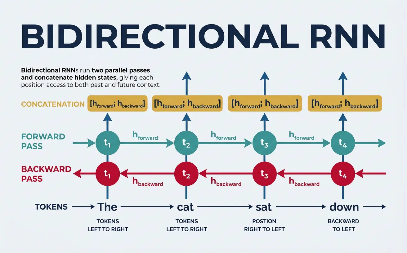
Standard RNNs process sequences in one direction—typically left to right—which means the hidden state at position t only contains information about tokens 0 to t. However, for many NLP tasks like named entity recognition or part-of-speech tagging, the meaning of a word depends on both its left and right context. Bidirectional RNNs address this by running two separate RNNs: one processing the sequence forward and one processing it backward.
The outputs from both directions are typically concatenated at each time step, doubling the hidden state size. This gives each position access to the entire sequence context. Bidirectional models are particularly powerful for tasks like sequence labeling, question answering, and sentiment analysis where full context is available at prediction time. However, they cannot be used for autoregressive generation (like language modeling) where future tokens are not available.
import torch
import torch.nn as nn

class BiLSTMClassifier(nn.Module):
    """
    Bidirectional LSTM for sequence classification.
    Useful for sentiment analysis, NER, etc.
    """

    def __init__(self, vocab_size, embedding_dim, hidden_size, num_classes,
                 num_layers=2, dropout=0.3):
        super().__init__()

        self.embedding = nn.Embedding(vocab_size, embedding_dim, padding_idx=0)
        self.dropout = nn.Dropout(dropout)

        self.bilstm = nn.LSTM(
            input_size=embedding_dim,
            hidden_size=hidden_size,
            num_layers=num_layers,
            batch_first=True,
            bidirectional=True,  # Key: bidirectional!
            dropout=dropout if num_layers > 1 else 0
        )

        # Output size is doubled due to bidirectional
        self.fc = nn.Linear(hidden_size * 2, num_classes)

    def forward(self, x, lengths=None):
        """
        Args:
            x: Token indices (batch_size, seq_length)
            lengths: Actual sequence lengths for masking (optional)

        Returns:
            logits: Classification logits (batch_size, num_classes)
        """
        embedded = self.dropout(self.embedding(x))

        # BiLSTM forward pass
        output, (h_n, c_n) = self.bilstm(embedded)
        # output shape: (batch, seq, hidden_size * 2)
        # h_n shape: (num_layers * 2, batch, hidden_size)

        # For classification, combine final hidden states from both directions
        # Forward direction: h_n[-2] (second to last)
        # Backward direction: h_n[-1] (last)
        forward_final = h_n[-2]  # (batch, hidden_size)
        backward_final = h_n[-1]  # (batch, hidden_size)

        # Concatenate
        combined = torch.cat([forward_final, backward_final], dim=1)
        # combined shape: (batch, hidden_size * 2)

        logits = self.fc(self.dropout(combined))

        return logits, output

# Example: Sentiment classification
vocab_size = 10000
embedding_dim = 128
hidden_size = 256
num_classes = 3  # Negative, Neutral, Positive

model = BiLSTMClassifier(vocab_size, embedding_dim, hidden_size, num_classes)

# Sample input
batch_size = 4
seq_length = 30
x = torch.randint(0, vocab_size, (batch_size, seq_length))

logits, hidden_states = model(x)

print(f"Input: {x.shape}")
print(f"Classification logits: {logits.shape}")
print(f"Hidden states at each position: {hidden_states.shape}")
import torch
import torch.nn as nn

class BiLSTMForNER(nn.Module):
    """
    Bidirectional LSTM for Named Entity Recognition (sequence labeling).
    Predicts a label for each token in the sequence.
    """

    def __init__(self, vocab_size, embedding_dim, hidden_size, num_tags,
                 num_layers=2, dropout=0.3):
        super().__init__()

        self.embedding = nn.Embedding(vocab_size, embedding_dim, padding_idx=0)
        self.dropout = nn.Dropout(dropout)

        self.bilstm = nn.LSTM(
            input_size=embedding_dim,
            hidden_size=hidden_size,
            num_layers=num_layers,
            batch_first=True,
            bidirectional=True,
            dropout=dropout if num_layers > 1 else 0
        )

        # Predict tag for each position
        self.fc = nn.Linear(hidden_size * 2, num_tags)

    def forward(self, x):
        """
        Args:
            x: Token indices (batch_size, seq_length)

        Returns:
            tag_logits: Logits for each position (batch_size, seq_length, num_tags)
        """
        embedded = self.dropout(self.embedding(x))

        # BiLSTM produces hidden states for each position
        output, _ = self.bilstm(embedded)
        # output: (batch, seq, hidden_size * 2)

        # Project to tag space for each position
        tag_logits = self.fc(self.dropout(output))
        # tag_logits: (batch, seq, num_tags)

        return tag_logits

    def predict(self, x):
        """Get predicted tags for input."""
        logits = self.forward(x)
        predictions = logits.argmax(dim=-1)
        return predictions

# Example: NER with BIO tagging
# Tags: O, B-PER, I-PER, B-ORG, I-ORG, B-LOC, I-LOC
tag_to_id = {'O': 0, 'B-PER': 1, 'I-PER': 2, 'B-ORG': 3, 'I-ORG': 4, 'B-LOC': 5, 'I-LOC': 6}
id_to_tag = {v: k for k, v in tag_to_id.items()}

vocab_size = 10000
embedding_dim = 128
hidden_size = 256
num_tags = len(tag_to_id)

model = BiLSTMForNER(vocab_size, embedding_dim, hidden_size, num_tags)

# Sample input
x = torch.randint(1, vocab_size, (2, 15))  # 2 sentences, length 15
tag_logits = model(x)
predictions = model.predict(x)

print(f"Input shape: {x.shape}")
print(f"Tag logits shape: {tag_logits.shape}")
print(f"Predictions shape: {predictions.shape}")
print(f"Sample predictions: {[id_to_tag[p.item()] for p in predictions[0][:5]]}")
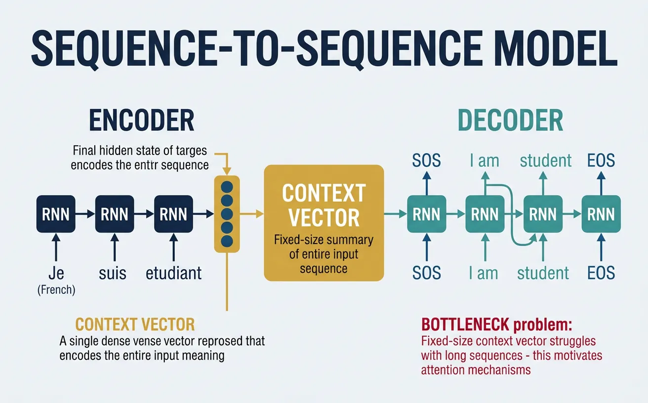
Sequence-to-Sequence Models
Sequence-to-Sequence (Seq2Seq) models, introduced by Sutskever et al. in 2014, are designed for tasks where both the input and output are sequences of potentially different lengths. The architecture consists of two main components: an encoder that reads the input sequence and compresses it into a fixed-length context vector, and a decoder that generates the output sequence one token at a time, conditioned on this context vector.
The encoder processes the entire input sequence and produces a final hidden state (and optionally cell state for LSTMs) that represents the "meaning" of the input. This context vector is used to initialize the decoder's hidden state. The decoder then generates tokens autoregressively: at each step, it takes the previous output token (or ground truth during training), updates its hidden state, and predicts the next token. This architecture is foundational for machine translation, summarization, and dialog systems.
Seq2Seq Architecture
flowchart LR
    subgraph ENC["ENCODER"]
        x1["x₁"] --> E1["LSTM"]
        x2["x₂"] --> E2["LSTM"]
        x3["x₃"] --> E3["LSTM"]
        EOS_in["<EOS>"] --> E4["LSTM"]
        E1 --> E2 --> E3 --> E4
    end

    E4 -->|"h_enc\n(context)"| CV(["Context\nVector"])

    subgraph DEC["DECODER"]
        SOS["<SOS>"] --> D1["LSTM"]
        D1 --> D2["LSTM"]
        D2 --> D3["LSTM"]
        D3 --> D4["LSTM"]
        D1 --> y1["y₁"]
        D2 --> y2["y₂"]
        D3 --> y3["y₃"]
        D4 --> EOS_out["<EOS>"]
    end

    CV -->|"init state"| D1
import torch
import torch.nn as nn
import torch.nn.functional as F

class Encoder(nn.Module):
    """
    LSTM encoder for Seq2Seq.
    """

    def __init__(self, vocab_size, embedding_dim, hidden_size, num_layers=2, dropout=0.3):
        super().__init__()
        self.hidden_size = hidden_size
        self.num_layers = num_layers

        self.embedding = nn.Embedding(vocab_size, embedding_dim, padding_idx=0)
        self.dropout = nn.Dropout(dropout)
        self.lstm = nn.LSTM(
            embedding_dim, hidden_size, num_layers,
            batch_first=True, dropout=dropout if num_layers > 1 else 0
        )

    def forward(self, src):
        """
        Args:
            src: Source sequence (batch_size, src_len)

        Returns:
            outputs: All hidden states (batch_size, src_len, hidden_size)
            hidden: Final (h_n, c_n) tuple
        """
        embedded = self.dropout(self.embedding(src))
        outputs, hidden = self.lstm(embedded)
        return outputs, hidden


class Decoder(nn.Module):
    """
    LSTM decoder for Seq2Seq.
    """

    def __init__(self, vocab_size, embedding_dim, hidden_size, num_layers=2, dropout=0.3):
        super().__init__()
        self.vocab_size = vocab_size
        self.hidden_size = hidden_size

        self.embedding = nn.Embedding(vocab_size, embedding_dim, padding_idx=0)
        self.dropout = nn.Dropout(dropout)
        self.lstm = nn.LSTM(
            embedding_dim, hidden_size, num_layers,
            batch_first=True, dropout=dropout if num_layers > 1 else 0
        )
        self.fc = nn.Linear(hidden_size, vocab_size)

    def forward(self, tgt, hidden):
        """
        Args:
            tgt: Target sequence (batch_size, tgt_len)
            hidden: Initial hidden state from encoder

        Returns:
            output: Predictions (batch_size, tgt_len, vocab_size)
            hidden: Final hidden state
        """
        embedded = self.dropout(self.embedding(tgt))
        output, hidden = self.lstm(embedded, hidden)
        output = self.fc(output)
        return output, hidden

    def generate_step(self, input_token, hidden):
        """Single decoding step for inference."""
        embedded = self.dropout(self.embedding(input_token))
        output, hidden = self.lstm(embedded, hidden)
        output = self.fc(output)
        return output, hidden


class Seq2Seq(nn.Module):
    """
    Complete Seq2Seq model combining encoder and decoder.
    """

    def __init__(self, encoder, decoder, device):
        super().__init__()
        self.encoder = encoder
        self.decoder = decoder
        self.device = device

    def forward(self, src, tgt, teacher_forcing_ratio=0.5):
        """
        Args:
            src: Source sequence (batch_size, src_len)
            tgt: Target sequence (batch_size, tgt_len)
            teacher_forcing_ratio: Probability of using ground truth

        Returns:
            outputs: Predictions (batch_size, tgt_len, vocab_size)
        """
        batch_size = src.size(0)
        tgt_len = tgt.size(1)
        vocab_size = self.decoder.vocab_size

        # Encode source
        _, hidden = self.encoder(src)

        # Prepare output tensor
        outputs = torch.zeros(batch_size, tgt_len, vocab_size, device=self.device)

        # First input to decoder is  token
        input_token = tgt[:, 0:1]  # (batch, 1)

        for t in range(1, tgt_len):
            output, hidden = self.decoder.generate_step(input_token, hidden)
            outputs[:, t:t+1, :] = output

            # Teacher forcing: use ground truth or predicted token
            teacher_force = torch.rand(1).item() < teacher_forcing_ratio
            top1 = output.argmax(dim=-1)  # Predicted token
            input_token = tgt[:, t:t+1] if teacher_force else top1

        return outputs

    def translate(self, src, max_len=50, sos_token=1, eos_token=2):
        """
        Translate source sequence (inference mode).
        """
        self.eval()
        with torch.no_grad():
            # Encode
            _, hidden = self.encoder(src)

            # Start with SOS token
            batch_size = src.size(0)
            input_token = torch.full((batch_size, 1), sos_token,
                                     dtype=torch.long, device=self.device)

            translated = [input_token.squeeze(1)]

            for _ in range(max_len):
                output, hidden = self.decoder.generate_step(input_token, hidden)
                predicted = output.argmax(dim=-1)
                translated.append(predicted.squeeze(1))

                # Stop if all sequences have generated EOS
                if (predicted == eos_token).all():
                    break

                input_token = predicted

            return torch.stack(translated, dim=1)

# Example usage
device = torch.device('cuda' if torch.cuda.is_available() else 'cpu')

src_vocab_size = 8000
tgt_vocab_size = 10000
embedding_dim = 256
hidden_size = 512
num_layers = 2

encoder = Encoder(src_vocab_size, embedding_dim, hidden_size, num_layers)
decoder = Decoder(tgt_vocab_size, embedding_dim, hidden_size, num_layers)
model = Seq2Seq(encoder, decoder, device).to(device)

# Sample input (batch of 4, source length 20, target length 25)
src = torch.randint(1, src_vocab_size, (4, 20)).to(device)
tgt = torch.randint(1, tgt_vocab_size, (4, 25)).to(device)

# Training forward pass
outputs = model(src, tgt, teacher_forcing_ratio=0.5)
print(f"Source: {src.shape}")
print(f"Target: {tgt.shape}")
print(f"Outputs: {outputs.shape}")

# Inference
translated = model.translate(src, max_len=30)
print(f"Translated: {translated.shape}")
The Information Bottleneck Problem
Limitation of basic Seq2Seq: The entire source sequence must be compressed into a single fixed-size context vector. For long sequences, this becomes a bottleneck—the encoder must cram all relevant information into one vector. This is why the attention mechanism (covered in Part 8) was introduced: it allows the decoder to look at different parts of the source sequence at each decoding step, eliminating the bottleneck.
Practical Implementation
Let's build a complete, practical example: a character-level language model using LSTMs. This model learns to predict the next character given a sequence of characters, which can be used to generate text in the style of the training data. Character-level models are simpler to implement (no tokenization needed) and provide good insight into how language models work.
import torch
import torch.nn as nn
import torch.optim as optim
from torch.utils.data import Dataset, DataLoader
import numpy as np

class CharDataset(Dataset):
    """Dataset for character-level language modeling."""

    def __init__(self, text, seq_length=100):
        self.seq_length = seq_length

        # Build character vocabulary
        self.chars = sorted(list(set(text)))
        self.char_to_idx = {c: i for i, c in enumerate(self.chars)}
        self.idx_to_char = {i: c for i, c in enumerate(self.chars)}
        self.vocab_size = len(self.chars)

        # Encode entire text
        self.encoded = torch.tensor([self.char_to_idx[c] for c in text], dtype=torch.long)

    def __len__(self):
        return len(self.encoded) - self.seq_length

    def __getitem__(self, idx):
        x = self.encoded[idx:idx + self.seq_length]
        y = self.encoded[idx + 1:idx + self.seq_length + 1]
        return x, y

    def decode(self, indices):
        """Convert indices back to string."""
        return ''.join([self.idx_to_char[i.item()] for i in indices])


class CharLSTM(nn.Module):
    """Character-level LSTM language model."""

    def __init__(self, vocab_size, embedding_dim=64, hidden_size=256, num_layers=2, dropout=0.3):
        super().__init__()
        self.hidden_size = hidden_size
        self.num_layers = num_layers

        self.embedding = nn.Embedding(vocab_size, embedding_dim)
        self.lstm = nn.LSTM(
            embedding_dim, hidden_size, num_layers,
            batch_first=True, dropout=dropout if num_layers > 1 else 0
        )
        self.dropout = nn.Dropout(dropout)
        self.fc = nn.Linear(hidden_size, vocab_size)

    def forward(self, x, hidden=None):
        embedded = self.embedding(x)
        output, hidden = self.lstm(embedded, hidden)
        output = self.dropout(output)
        logits = self.fc(output)
        return logits, hidden

    def init_hidden(self, batch_size, device):
        h0 = torch.zeros(self.num_layers, batch_size, self.hidden_size, device=device)
        c0 = torch.zeros(self.num_layers, batch_size, self.hidden_size, device=device)
        return (h0, c0)

    def generate(self, dataset, seed_text, length=200, temperature=0.8, device='cpu'):
        """Generate text given a seed string."""
        self.eval()

        # Encode seed text
        encoded = torch.tensor([dataset.char_to_idx[c] for c in seed_text],
                               dtype=torch.long, device=device).unsqueeze(0)

        hidden = self.init_hidden(1, device)
        generated = list(seed_text)

        # Process seed to get initial hidden state
        with torch.no_grad():
            for i in range(len(seed_text) - 1):
                _, hidden = self.forward(encoded[:, i:i+1], hidden)

            # Generate new characters
            current_char = encoded[:, -1:]

            for _ in range(length):
                output, hidden = self.forward(current_char, hidden)

                # Apply temperature sampling
                probs = torch.softmax(output[0, 0] / temperature, dim=0)
                next_idx = torch.multinomial(probs, 1).item()

                generated.append(dataset.idx_to_char[next_idx])
                current_char = torch.tensor([[next_idx]], device=device)

        return ''.join(generated)


# Example: Train on sample text
sample_text = """
The quick brown fox jumps over the lazy dog. Natural language processing is fascinating.
Machine learning models can learn patterns from text data. Recurrent neural networks
process sequences one step at a time. Long Short-Term Memory networks solve the
vanishing gradient problem. The hidden state captures information about the sequence.
""" * 100  # Repeat for more data

# Create dataset and dataloader
dataset = CharDataset(sample_text, seq_length=50)
dataloader = DataLoader(dataset, batch_size=32, shuffle=True, drop_last=True)

print(f"Vocabulary size: {dataset.vocab_size}")
print(f"Characters: {''.join(dataset.chars[:30])}...")
print(f"Total sequences: {len(dataset)}")

# Create model
device = torch.device('cuda' if torch.cuda.is_available() else 'cpu')
model = CharLSTM(dataset.vocab_size).to(device)

# Training loop (abbreviated for demo)
criterion = nn.CrossEntropyLoss()
optimizer = optim.Adam(model.parameters(), lr=0.002)

model.train()
for epoch in range(3):  # More epochs needed for good results
    total_loss = 0
    for batch_idx, (x, y) in enumerate(dataloader):
        x, y = x.to(device), y.to(device)

        optimizer.zero_grad()
        output, _ = model(x)
        loss = criterion(output.view(-1, dataset.vocab_size), y.view(-1))
        loss.backward()
        torch.nn.utils.clip_grad_norm_(model.parameters(), 5.0)
        optimizer.step()

        total_loss += loss.item()

    print(f"Epoch {epoch+1}, Avg Loss: {total_loss/len(dataloader):.4f}")

# Generate sample text
generated = model.generate(dataset, "The quick", length=100, temperature=0.8, device=device)
print(f"\nGenerated text:\n{generated}")
import torch
import torch.nn as nn
import torch.optim as optim

# Complete training pipeline for word-level language model
class WordLevelLM(nn.Module):
    """Word-level LSTM language model with proper training utilities."""

    def __init__(self, vocab_size, embedding_dim=256, hidden_size=512,
                 num_layers=2, dropout=0.5, tie_weights=True):
        super().__init__()
        self.hidden_size = hidden_size
        self.num_layers = num_layers

        self.embedding = nn.Embedding(vocab_size, embedding_dim)
        self.dropout = nn.Dropout(dropout)
        self.lstm = nn.LSTM(
            embedding_dim, hidden_size, num_layers,
            batch_first=True, dropout=dropout
        )
        self.fc = nn.Linear(hidden_size, vocab_size)

        # Weight tying (reduces parameters, often improves performance)
        if tie_weights and embedding_dim == hidden_size:
            self.fc.weight = self.embedding.weight

        self.init_weights()

    def init_weights(self):
        """Initialize weights for better training."""
        init_range = 0.1
        self.embedding.weight.data.uniform_(-init_range, init_range)
        self.fc.bias.data.zero_()
        self.fc.weight.data.uniform_(-init_range, init_range)

    def forward(self, x, hidden=None):
        embedded = self.dropout(self.embedding(x))
        output, hidden = self.lstm(embedded, hidden)
        output = self.dropout(output)
        logits = self.fc(output)
        return logits, hidden

    def init_hidden(self, batch_size, device):
        h = torch.zeros(self.num_layers, batch_size, self.hidden_size, device=device)
        c = torch.zeros(self.num_layers, batch_size, self.hidden_size, device=device)
        return (h, c)


def train_epoch(model, dataloader, criterion, optimizer, clip_grad, device):
    """Train for one epoch."""
    model.train()
    total_loss = 0
    hidden = None

    for batch_idx, (x, y) in enumerate(dataloader):
        x, y = x.to(device), y.to(device)

        # Detach hidden state to prevent BPTT across batches
        if hidden is not None:
            hidden = (hidden[0].detach(), hidden[1].detach())

        optimizer.zero_grad()
        output, hidden = model(x, hidden)

        loss = criterion(output.view(-1, output.size(-1)), y.view(-1))
        loss.backward()

        # Gradient clipping
        torch.nn.utils.clip_grad_norm_(model.parameters(), clip_grad)

        optimizer.step()
        total_loss += loss.item()

    return total_loss / len(dataloader)


def evaluate(model, dataloader, criterion, device):
    """Evaluate model on validation/test set."""
    model.eval()
    total_loss = 0
    hidden = None

    with torch.no_grad():
        for x, y in dataloader:
            x, y = x.to(device), y.to(device)
            output, hidden = model(x, hidden)
            loss = criterion(output.view(-1, output.size(-1)), y.view(-1))
            total_loss += loss.item()

    return total_loss / len(dataloader)


# Example usage
vocab_size = 10000
model = WordLevelLM(vocab_size)
print(f"Model parameters: {sum(p.numel() for p in model.parameters()):,}")

# Count parameters by component
emb_params = sum(p.numel() for p in model.embedding.parameters())
lstm_params = sum(p.numel() for p in model.lstm.parameters())
fc_params = sum(p.numel() for p in model.fc.parameters())

print(f"  Embedding: {emb_params:,}")
print(f"  LSTM: {lstm_params:,}")
print(f"  Output layer: {fc_params:,}")
Training Tips for RNN Language Models
Key practices for successful training: 1) Use gradient clipping (typically max_norm=5.0) to prevent exploding gradients. 2) Initialize forget gate bias to 1.0 for LSTMs. 3) Apply dropout between LSTM layers and before the output layer. 4) Use learning rate scheduling (reduce on plateau). 5) Detach hidden states when using truncated BPTT. 6) Consider weight tying between embedding and output layers to reduce parameters and regularize.
import torch
import torch.nn as nn

# Stacked and Residual RNNs for deeper models
class ResidualLSTM(nn.Module):
    """
    LSTM with residual connections for training deeper models.
    """

    def __init__(self, input_size, hidden_size, num_layers=4, dropout=0.3):
        super().__init__()
        self.num_layers = num_layers

        # First layer may have different input size
        self.layers = nn.ModuleList()
        self.dropouts = nn.ModuleList()

        for i in range(num_layers):
            in_size = input_size if i == 0 else hidden_size
            self.layers.append(nn.LSTM(in_size, hidden_size, num_layers=1, batch_first=True))
            self.dropouts.append(nn.Dropout(dropout))

        # Projection if input_size != hidden_size
        self.input_proj = nn.Linear(input_size, hidden_size) if input_size != hidden_size else None

    def forward(self, x, hiddens=None):
        """
        Args:
            x: Input (batch, seq, input_size)
            hiddens: List of (h, c) tuples for each layer

        Returns:
            output: (batch, seq, hidden_size)
            hiddens: List of new (h, c) tuples
        """
        if hiddens is None:
            hiddens = [None] * self.num_layers

        new_hiddens = []
        output = x

        for i, (lstm, dropout) in enumerate(zip(self.layers, self.dropouts)):
            residual = output

            # Project residual if needed (first layer)
            if i == 0 and self.input_proj is not None:
                residual = self.input_proj(residual)

            output, hidden = lstm(output, hiddens[i])
            output = dropout(output)

            # Add residual connection (skip first layer if sizes don't match)
            if i > 0 or self.input_proj is not None:
                output = output + residual

            new_hiddens.append(hidden)

        return output, new_hiddens


# Example
batch_size = 4
seq_length = 50
input_size = 128
hidden_size = 256

model = ResidualLSTM(input_size, hidden_size, num_layers=4)
x = torch.randn(batch_size, seq_length, input_size)

output, hiddens = model(x)
print(f"Input: {x.shape}")
print(f"Output: {output.shape}")
print(f"Number of hidden states: {len(hiddens)}")
Conclusion & Next Steps
In this comprehensive guide, we've explored the evolution of recurrent architectures for sequence modeling. We started with vanilla RNNs, understanding their elegant simplicity but also their fundamental limitation: the vanishing gradient problem that prevents learning long-range dependencies. We then examined how LSTMs solve this problem through their gating mechanisms and cell state—a dedicated pathway that allows gradients to flow unimpeded across many time steps.
We also covered GRUs as a simpler alternative to LSTMs, bidirectional RNNs for tasks requiring full context, and Seq2Seq models for mapping sequences to sequences. These architectures formed the foundation of NLP before the transformer revolution and remain relevant for many applications, especially when computational resources are limited or when the sequential nature of data is particularly important.
Key Takeaways
- Vanilla RNNs process sequences but suffer from vanishing/exploding gradients, limiting them to short-range dependencies (~10-20 steps)
- LSTMs introduce cell state and three gates (forget, input, output) to control information flow and enable long-range learning
- GRUs simplify LSTMs with two gates (update, reset) and ~25% fewer parameters while maintaining similar performance
- Bidirectional RNNs process sequences in both directions, providing full context for each position
- Seq2Seq models combine encoder and decoder for variable-length input-to-output mapping
- Practical tips: Use gradient clipping, forget gate bias initialization, weight tying, and truncated BPTT