Introduction to Text Representation
Before applying machine learning to text, we need to convert words into numerical vectors. This third part covers classical text representation methods that laid the foundation for modern NLP.
Key Insight
Classical text representations like TF-IDF are still valuable for many tasks and serve as strong baselines before deploying complex neural models.
NLP Mastery
NLP Fundamentals & Linguistic Basics
Phonology, morphology, syntax, semantics, pragmaticsTokenization & Text Cleaning
Subword tokenization, BPE, stopwords, normalizationText Representation & Feature Engineering
Bag-of-words, TF-IDF, feature extraction, vectorizationWord Embeddings
Word2Vec, GloVe, FastText, embedding spaces, analogiesStatistical Language Models & N-grams
Probability chains, smoothing, perplexity, Markov modelsNeural Networks for NLP
Feedforward nets, backpropagation, activation functionsRNNs, LSTMs & GRUs
Sequence modeling, vanishing gradients, gated architecturesTransformers & Attention Mechanism
Self-attention, multi-head attention, positional encodingPretrained Language Models & Transfer Learning
BERT, RoBERTa, fine-tuning, feature extractionGPT Models & Text Generation
Autoregressive generation, prompting, GPT architectureCore NLP Tasks
NER, POS tagging, sentiment analysis, text classificationAdvanced NLP Tasks
Question answering, summarization, machine translationMultilingual & Cross-lingual NLP
mBERT, XLM-R, zero-shot transfer, language diversityEvaluation, Ethics & Responsible NLP
BLEU, ROUGE, bias detection, fairness, responsible AINLP Systems, Optimization & Production
Model serving, quantization, distillation, deploymentCutting-Edge & Research Topics
LLMs, multimodal NLP, reasoning, emerging researchOne-Hot Encoding
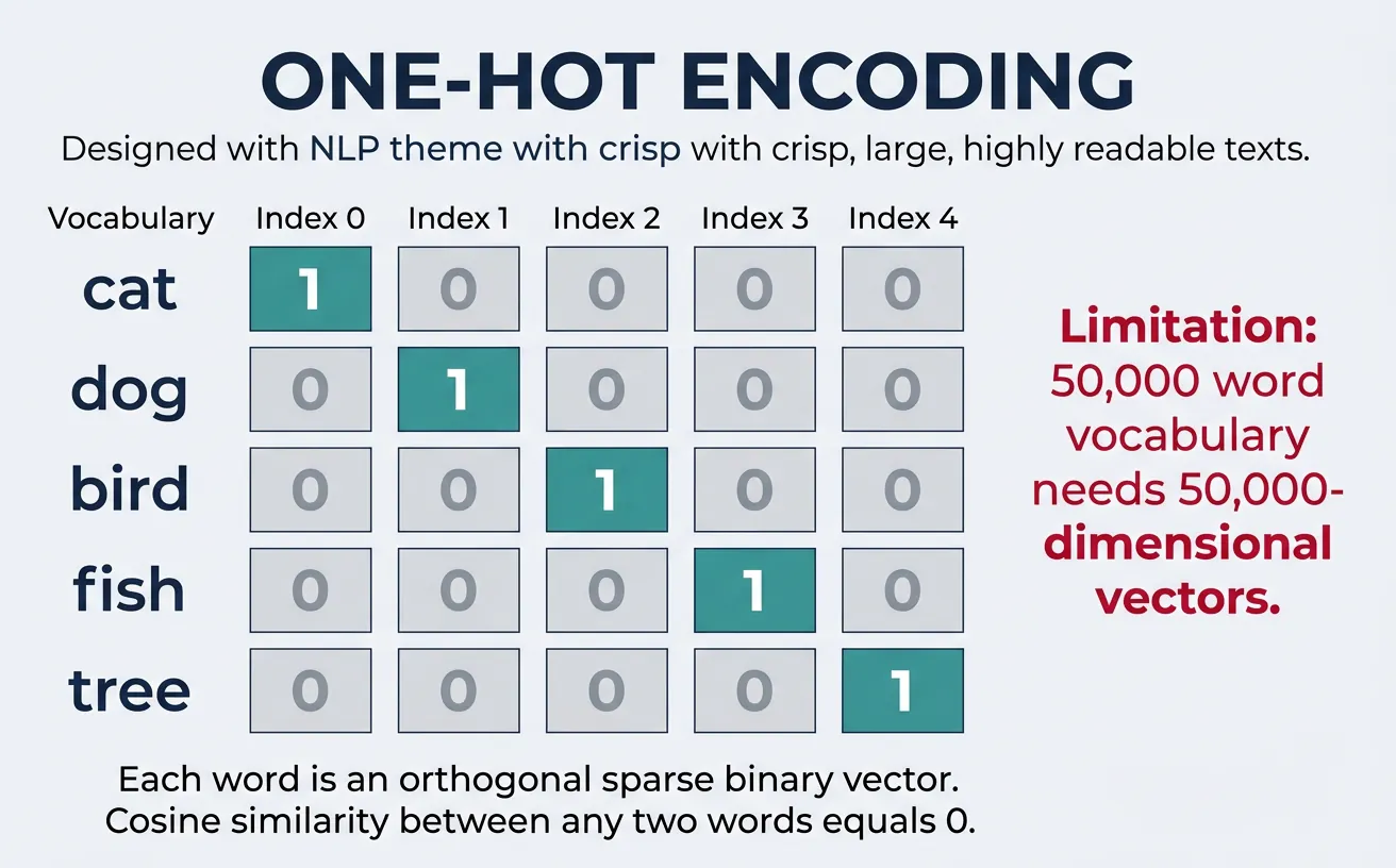
One-hot encoding is the simplest form of text representation where each word in the vocabulary is represented as a binary vector with exactly one element set to 1 and all others set to 0. The position of the "1" corresponds to the word's index in the vocabulary. For a vocabulary of size V, each word becomes a V-dimensional vector that uniquely identifies it.
Consider a vocabulary of ["cat", "dog", "bird"]. The word "cat" would be represented as [1, 0, 0], "dog" as [0, 1, 0], and "bird" as [0, 0, 1]. This representation treats each word as completely independent—there's no notion that "cat" and "dog" are both animals while "bird" is different. The orthogonality of vectors means cosine similarity between any two different words is always zero.
Why One-Hot Encoding Matters
One-hot encoding provides a foundation for understanding more advanced representations. While impractical for large vocabularies, it's the conceptual basis for neural network input layers and helps illustrate why we need denser, more meaningful representations like word embeddings.
import numpy as np
from sklearn.preprocessing import LabelEncoder, OneHotEncoder

# Sample vocabulary
vocabulary = ['apple', 'banana', 'cherry', 'date', 'elderberry']

# Create one-hot encoder
label_encoder = LabelEncoder()
integer_encoded = label_encoder.fit_transform(vocabulary)
print("Label Encoded:", integer_encoded)
# Output: [0 1 2 3 4]

# Reshape for one-hot encoding
integer_encoded = integer_encoded.reshape(-1, 1)
onehot_encoder = OneHotEncoder(sparse_output=False)
onehot_encoded = onehot_encoder.fit_transform(integer_encoded)

print("\nOne-Hot Encoded Vectors:")
for word, vector in zip(vocabulary, onehot_encoded):
    print(f"  {word:12} -> {vector}")
# apple        -> [1. 0. 0. 0. 0.]
# banana       -> [0. 1. 0. 0. 0.]
# cherry       -> [0. 0. 1. 0. 0.]
# date         -> [0. 0. 0. 1. 0.]
# elderberry   -> [0. 0. 0. 0. 1.]
The Dimensionality Explosion Problem
The primary limitation of one-hot encoding is dimensionality explosion. To understand why, start small. With a 5-word vocabulary, each word becomes a 5-number vector with exactly one 1 and the rest 0:
import numpy as np

# Tiny vocabulary of 5 words
vocab = ["cat", "dog", "mat", "sat", "the"]
vocab_size = len(vocab)
word_to_idx = {word: idx for idx, word in enumerate(vocab)}

# Build one-hot vectors
one_hot = np.eye(vocab_size, dtype=int)

for word, idx in word_to_idx.items():
    print(f'"{word}" → {one_hot[idx].tolist()}')

# Each vector: 5 numbers, 4 are wasted zeros
total_numbers = vocab_size * vocab_size
zeros = total_numbers - vocab_size
print(f"\nTotal numbers stored: {total_numbers}")
print(f"Zeros (wasted): {zeros}  ({zeros/total_numbers*100:.0f}% of storage)")
Now scale that to a real English vocabulary of 50,000 words. Every single word becomes a 50,000-number vector where 49,999 of those numbers are zero — 99.998% of the storage is wasted:
import numpy as np

# Compare vector sizes at different vocabulary scales
vocab_sizes = [5, 1_000, 50_000]

print(f"{'Vocabulary':>12}  {'Vector size':>12}  {'Zeros per vector':>18}  {'Wasted %':>10}")
print("-" * 60)
for v in vocab_sizes:
    zeros = v - 1
    pct = zeros / v * 100
    print(f"{v:>12,}  {v:>12,}  {zeros:>18,}  {pct:>9.3f}%")
Storage Cost: One Six-Word Sentence
The sentence "The cat sat on the mat" is just 6 words. With a 50,000-word vocabulary:
- Each word → 50,000 numbers
- 6 words → 6 × 50,000 = 300,000 numbers
- At 4 bytes per float → ~1.2 MB for one sentence
- A dataset of 1 million sentences → ~1.2 TB of mostly zeros
# Storage calculation for one-hot encoding
vocab_size = 50_000
sentence = ["the", "cat", "sat", "on", "the", "mat"]
num_words = len(sentence)
bytes_per_float = 4  # 32-bit float

numbers_stored = num_words * vocab_size
bytes_used = numbers_stored * bytes_per_float
mb_used = bytes_used / (1024 ** 2)

print(f"Sentence: {' '.join(sentence)!r}")
print(f"Words: {num_words}")
print(f"Numbers stored: {numbers_stored:,}  ({num_words} × {vocab_size:,})")
print(f"Storage: {bytes_used:,} bytes = {mb_used:.2f} MB")

# Scale to a dataset
num_sentences = 1_000_000
total_gb = (mb_used * num_sentences) / 1024
print(f"\n1 million such sentences: {total_gb:,.0f} GB = {total_gb/1024:.1f} TB")
print(f"(Almost entirely zeros — {(vocab_size - 1) / vocab_size * 100:.3f}% of each vector)")
No Semantic Relationships
Beyond the storage problem, one-hot vectors are semantically blind. Every word is equally distant from every other word. The model has no way to know that "cat" and "dog" are both animals, or that "sat" and "ran" are both verbs:
import numpy as np

# One-hot vectors for 5 words
vocab = ["cat", "dog", "mat", "sat", "the"]
word_to_idx = {word: idx for idx, word in enumerate(vocab)}
one_hot = np.eye(len(vocab))

def cosine_similarity(a, b):
    """Cosine similarity: 1.0 = identical, 0.0 = completely different."""
    return np.dot(a, b) / (np.linalg.norm(a) * np.linalg.norm(b))

cat = one_hot[word_to_idx["cat"]]
dog = one_hot[word_to_idx["dog"]]
mat = one_hot[word_to_idx["mat"]]

sim_cat_dog = cosine_similarity(cat, dog)
sim_cat_mat = cosine_similarity(cat, mat)

print(f"Similarity(cat, dog) = {sim_cat_dog:.1f}  ← both animals, but model sees 0")
print(f"Similarity(cat, mat) = {sim_cat_mat:.1f}  ← completely unrelated, also 0")
print("\nOne-hot encoding treats every word as equally different from every other word.")
print("'cat'/'dog' distance == 'cat'/'mat' distance — semantics are invisible.")
The Fix: Word Embeddings
Instead of 50,000-dimensional sparse vectors, word embeddings map each word to a small dense vector (~300 numbers) where all values are meaningful — and similar words end up with similar vectors:
| One-hot | Word embedding | |
|---|---|---|
| Vector size | 50,000 | 300 |
| Zeros per vector | 49,999 | 0 |
| Captures meaning | ✗ | ✓ |
| Storage (1M sentences) | ~1.2 TB | ~7 GB |
| Compression ratio | — | ~167× smaller |
One-Hot Encoding for Sentences
import numpy as np

def one_hot_encode_sentence(sentence, vocab_to_idx):
    """Encode a sentence as sequence of one-hot vectors."""
    words = sentence.lower().split()
    vocab_size = len(vocab_to_idx)
    encoded = np.zeros((len(words), vocab_size))

    for i, word in enumerate(words):
        if word in vocab_to_idx:
            encoded[i, vocab_to_idx[word]] = 1
    return encoded

# Build vocabulary from corpus
corpus = ["the cat sat on the mat", "the dog ran in the park"]
all_words = set(' '.join(corpus).split())
vocab_to_idx = {word: idx for idx, word in enumerate(sorted(all_words))}

print("Vocabulary:", vocab_to_idx)
# {'cat': 0, 'dog': 1, 'in': 2, 'mat': 3, 'on': 4, 'park': 5, 'ran': 6, 'sat': 7, 'the': 8}

# Encode a sentence
sentence = "the cat sat"
encoded = one_hot_encode_sentence(sentence, vocab_to_idx)
print(f"\nSentence: '{sentence}'")
print("Shape:", encoded.shape)  # (3, 9)
print("Encoded:")
print(encoded)
Bag of Words (BoW)
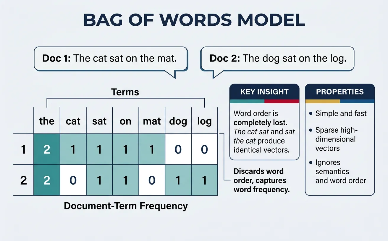
The Bag of Words (BoW) model represents a document as an unordered collection of words, disregarding grammar and word order while keeping track of word frequency. Each document becomes a vector where each dimension corresponds to a vocabulary term, and the value represents how many times that term appears in the document. This simple yet powerful representation enables quantitative comparison between documents.
The name "bag of words" comes from the metaphor of throwing all words from a document into a bag—you know what words are present and how many of each, but you lose all information about their original order. Despite this limitation, BoW has proven remarkably effective for tasks like document classification, sentiment analysis, and information retrieval.
Implementation
Scikit-learn's CountVectorizer provides an efficient implementation of BoW that handles tokenization, vocabulary building, and document encoding in a single pipeline. By default, it converts text to lowercase and removes single-character tokens, but these behaviors are fully configurable.
fit vs transform vs fit_transform
You'll see these three methods throughout this article. They have distinct roles:
fit(data)— Learns the vocabulary from the data (scans all words, assigns each an index). Returns the vectorizer itself. Does not produce a matrix. Use when you only need the vocabulary.transform(data)— Converts text into vectors using an already-learned vocabulary. Fails if called beforefit. Use on new/unseen data after fitting on training data.fit_transform(data)— Does both steps in one call: learns the vocabulary then immediately returns the matrix. More efficient than calling them separately. Use on your training data.
from sklearn.feature_extraction.text import CountVectorizer

train_docs = ["machine learning is great", "deep learning is powerful"]
test_docs  = ["machine learning helps everyone"]

vec = CountVectorizer()

# --- fit only ---
# Learns vocabulary: {'deep':0, 'great':1, 'is':2, 'learning':3, 'machine':4, 'powerful':5}
vec.fit(train_docs)
print("Vocabulary:", vec.vocabulary_)       # dict of word → column index
# No matrix produced yet

# --- transform (uses the vocabulary already learned by fit) ---
train_matrix = vec.transform(train_docs)    # train data → matrix
test_matrix  = vec.transform(test_docs)     # new data → same columns, same vocabulary
print("Train shape:", train_matrix.shape)   # (2, 6)
print("Test shape: ", test_matrix.shape)    # (1, 6) — same 6 columns

# --- fit_transform (fit + transform in one step, more efficient) ---
vec2 = CountVectorizer()
matrix = vec2.fit_transform(train_docs)     # equivalent to fit then transform
print("fit_transform shape:", matrix.shape) # (2, 6)

# IMPORTANT: Never fit on test data — it leaks information
# Wrong:  vec.fit_transform(test_docs)   ← creates a new vocabulary from test data
# Right:  vec.transform(test_docs)       ← reuses vocabulary learned from training
from sklearn.feature_extraction.text import CountVectorizer
import pandas as pd

# Sample documents
documents = [
    "Machine learning is fascinating and useful",
    "Deep learning is a subset of machine learning",
    "Natural language processing uses machine learning",
    "NLP is useful for text analysis"
]

# Create Bag of Words model
vectorizer = CountVectorizer()
bow_matrix = vectorizer.fit_transform(documents)

# Get feature names (vocabulary)
feature_names = vectorizer.get_feature_names_out()
print("Vocabulary:", list(feature_names))

# Convert to DataFrame for visualization
bow_df = pd.DataFrame(
    bow_matrix.toarray(),
    columns=feature_names,
    index=[f"Doc {i+1}" for i in range(len(documents))]
)
print("\nBag of Words Matrix:")
print(bow_df)

# Document similarity using dot product
from sklearn.metrics.pairwise import cosine_similarity
similarity = cosine_similarity(bow_matrix)
print("\nDocument Similarity Matrix:")
print(pd.DataFrame(similarity, index=bow_df.index, columns=bow_df.index).round(3))
The BoW representation allows us to perform document-level operations like finding similar documents, clustering related content, and training classifiers. The cosine similarity between BoW vectors provides a natural measure of document similarity that's robust to document length differences.
CountVectorizer Configuration Options
from sklearn.feature_extraction.text import CountVectorizer

documents = [
    "The quick brown fox jumps over the lazy dog",
    "A quick brown dog outpaces a lazy fox",
    "Machine learning and deep learning are related"
]

# Basic vectorizer
basic_vec = CountVectorizer()
print("Basic vocabulary size:", len(basic_vec.fit(documents).vocabulary_))

# With stop words removed
no_stop_vec = CountVectorizer(stop_words='english')
print("Without stop words:", len(no_stop_vec.fit(documents).vocabulary_))

# With minimum document frequency
min_df_vec = CountVectorizer(min_df=2)  # Word must appear in at least 2 docs
print("min_df=2 vocabulary:", list(min_df_vec.fit(documents).vocabulary_.keys()))

# With n-gram range (unigrams and bigrams)
ngram_vec = CountVectorizer(ngram_range=(1, 2))
ngram_matrix = ngram_vec.fit_transform(documents)
print("Unigrams + Bigrams features:", ngram_matrix.shape[1])

# With maximum features
max_feat_vec = CountVectorizer(max_features=10)
print("Top 10 features:", list(max_feat_vec.fit(documents).vocabulary_.keys()))

# Binary BoW (presence/absence only)
binary_vec = CountVectorizer(binary=True)
binary_matrix = binary_vec.fit_transform(documents)
print("\nBinary BoW (first doc):", binary_matrix.toarray()[0][:10])
What does binary=True do in CountVectorizer?
By default, CountVectorizer stores raw term counts — if "cat" appears 3 times in a document, the cell value is 3. With binary=True, every non-zero count is replaced by 1, so "cat cat cat" and "cat" both produce the same value of 1. The vector simply records whether a word is present, not how many times.
When is it useful? Short documents where high frequency is noise rather than signal (e.g., tweets, one-line reviews), or when you're feeding the matrix into a Bernoulli Naïve Bayes classifier, which explicitly assumes binary features and performs better with them than with raw counts.
Limitations
While BoW is simple and effective for many tasks, it has significant limitations. Loss of word order means "dog bites man" and "man bites dog" have identical representations. Loss of context prevents distinguishing between different meanings of the same word. Vocabulary scaling creates increasingly sparse vectors as vocabulary grows. No semantic similarity means synonyms like "happy" and "joyful" are treated as completely unrelated.
BoW Limitations Summary
| Limitation | Impact | Mitigation |
|---|---|---|
| No word order | "not good" = "good not" | Use N-grams |
| High dimensionality | Sparse, memory-intensive | Dimensionality reduction |
| No semantics | Synonyms unrelated | Word embeddings |
| Equal word importance | Common words dominate | TF-IDF weighting |
Measuring Similarity: Cosine Similarity
Once documents or words are represented as numerical vectors, we need a reliable way to measure how similar two vectors are. The most widely used metric in NLP is cosine similarity, which measures the cosine of the angle between two vectors in high-dimensional space. It tells you whether two vectors point in roughly the same direction, regardless of their magnitude (length).
The Formula
For two vectors A and B, cosine similarity is defined as:
cos(θ) = (A · B) / (||A|| × ||B||)
- A · B (dot product) = sum of element-wise products
- ||A|| = Euclidean norm (magnitude) of vector A
- Range: −1 (opposite) to +1 (identical direction). For non-negative vectors like BoW or TF-IDF the range is 0 to +1.
Why cosine over Euclidean distance? In text, document length varies enormously. A 10-page article about "machine learning" will have much larger raw word counts than a 2-sentence abstract on the same topic, so their Euclidean distance would be large even though they discuss the same subject. Cosine similarity ignores magnitude and focuses on direction, making it robust to document length differences.
Cosine Similarity vs Euclidean Distance
| Property | Cosine Similarity | Euclidean Distance |
|---|---|---|
| Measures | Angle between vectors (direction) | Straight-line distance (magnitude) |
| Range | −1 to +1 (0 to +1 for positive vectors) | 0 to ∞ |
| Length-sensitive? | No — normalizes by magnitude | Yes — longer documents appear more distant |
| Best for | Comparing text, high-dimensional sparse vectors | Low-dimensional, similar-scale data |
| Interpretation | 1 = identical direction, 0 = unrelated | 0 = identical, larger = more different |
# Understanding cosine similarity step by step
import numpy as np

def cosine_similarity_manual(vec_a, vec_b):
    """Compute cosine similarity from scratch."""
    dot_product = np.dot(vec_a, vec_b)
    norm_a = np.linalg.norm(vec_a)
    norm_b = np.linalg.norm(vec_b)
    return dot_product / (norm_a * norm_b)

# Example 1: Two documents about similar topics
doc_ML = np.array([3, 2, 0, 1, 0])   # "machine learning data model algorithm"
doc_AI = np.array([2, 1, 0, 1, 1])   # "machine learning neural model network"
doc_cook = np.array([0, 0, 3, 0, 0]) # "recipe recipe recipe"

print("Cosine similarities:")
print(f"  ML vs AI:      {cosine_similarity_manual(doc_ML, doc_AI):.4f}")  # ~0.89 (similar)
print(f"  ML vs Cooking:  {cosine_similarity_manual(doc_ML, doc_cook):.4f}")  # 0.0 (unrelated)
print(f"  AI vs Cooking:  {cosine_similarity_manual(doc_AI, doc_cook):.4f}")  # 0.0 (unrelated)

# Example 2: Magnitude doesn't matter
short_doc = np.array([1, 1, 0])   # short article about topic A
long_doc  = np.array([5, 5, 0])   # long article about topic A (same proportions)
diff_doc  = np.array([0, 0, 3])   # article about topic B

print("\nLength invariance:")
print(f"  Short vs Long (same topic): {cosine_similarity_manual(short_doc, long_doc):.4f}")  # 1.0
print(f"  Short vs Different topic:   {cosine_similarity_manual(short_doc, diff_doc):.4f}")  # 0.0

# Euclidean distance would incorrectly show short and long as very different:
euclidean = np.linalg.norm(short_doc - long_doc)
print(f"  Euclidean (short vs long): {euclidean:.2f} (misleadingly large!)")
# Practical usage with scikit-learn
from sklearn.feature_extraction.text import TfidfVectorizer
from sklearn.metrics.pairwise import cosine_similarity
import numpy as np
# Four documents
documents = [
"Machine learning algorithms detect patterns in data",
"Deep learning neural networks learn representations",
"Baking bread requires flour yeast and patience",
"Supervised learning models predict outcomes from data"
]
# Convert to TF-IDF vectors
vectorizer = TfidfVectorizer()
tfidf_matrix = vectorizer.fit_transform(documents)
# Compute pairwise cosine similarity
sim_matrix = cosine_similarity(tfidf_matrix)
print("Pairwise Cosine Similarity:\n")
for i in range(len(documents)):
for j in range(i + 1, len(documents)):
print(f" Doc {i+1} vs Doc {j+1}: {sim_matrix[i][j]:.3f}")
# Doc 1 vs 2 ~0.15 (both ML), Doc 1 vs 3 ~0.00 (unrelated),
# Doc 1 vs 4 ~0.30 (very similar)
# Find most similar document to a query
query = "pattern recognition using neural networks"
query_vec = vectorizer.transform([query])
scores = cosine_similarity(query_vec, tfidf_matrix).flatten()
print("\nQuery:", query)
for idx in np.argsort(scores)[::-1]:
print(f" [{scores[idx]:.3f}] {documents[idx]}")Where Cosine Similarity Appears Throughout NLP
- Information retrieval: Ranking search results by query-document similarity
- Word embeddings: Finding semantically similar words (king − man + woman ≈ queen)
- Document clustering: Grouping similar articles, emails, or reviews
- Duplicate detection: Identifying near-duplicate content or plagiarism
- Recommendation systems: Suggesting content similar to what a user liked
- BERTScore: Evaluating text generation quality using contextual embedding similarity
TF-IDF
TF-IDF (Term Frequency-Inverse Document Frequency) is a numerical statistic that reflects how important a word is to a document within a collection. Unlike raw word counts, TF-IDF balances term frequency against document frequency, giving higher weight to words that are frequent in a specific document but rare across the corpus. This makes it invaluable for document retrieval, keyword extraction, and text classification.
The intuition behind TF-IDF is straightforward: words that appear frequently in a document are likely relevant to its content, but words that appear in many documents (like "the" or "is") carry less discriminative information. By multiplying term frequency by inverse document frequency, we amplify distinctive terms while dampening common ones.
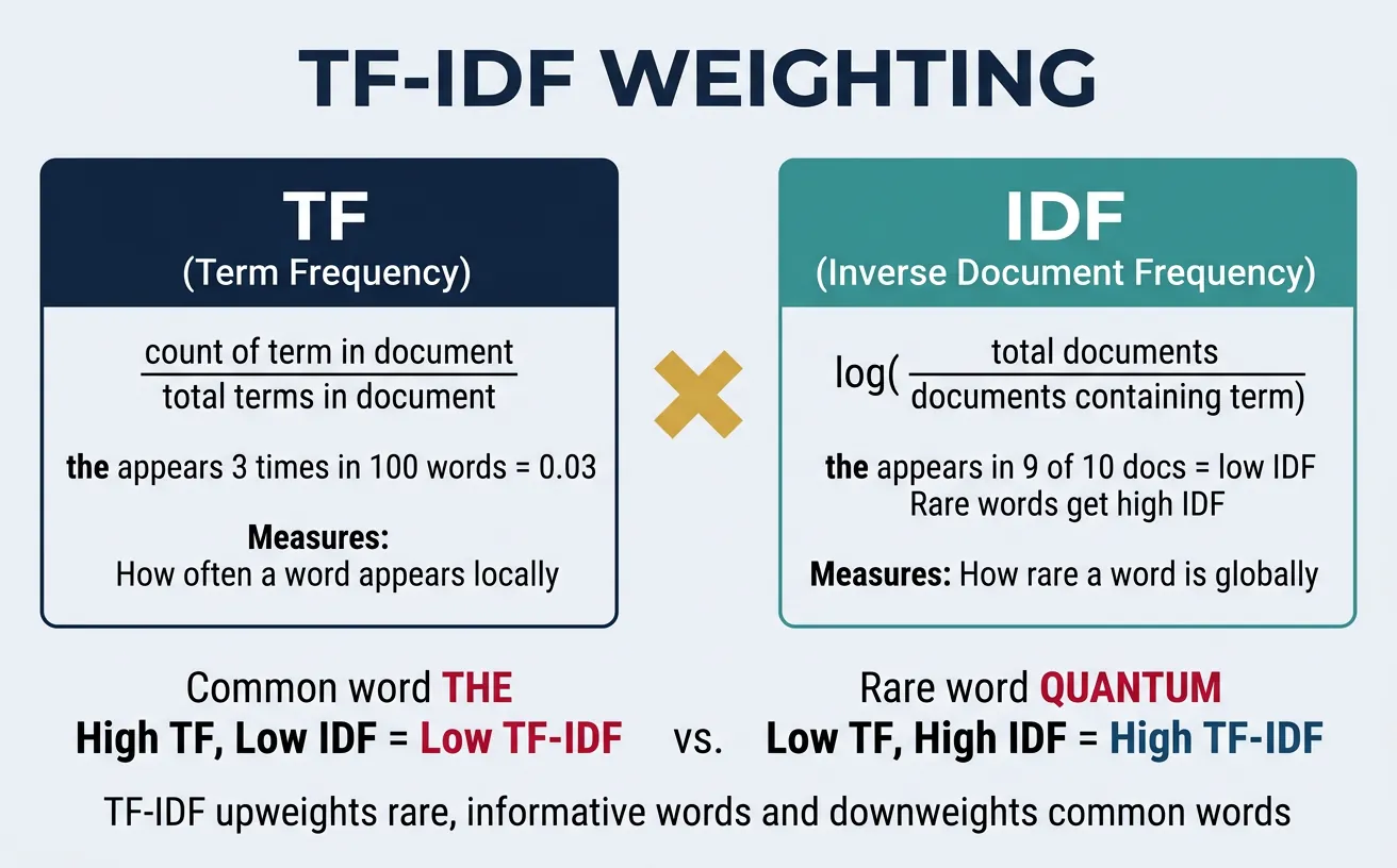
Term Frequency
Term Frequency (TF) measures how often a term appears in a document. The simplest form is the raw count, but this favors longer documents. Common normalization approaches include dividing by document length or taking the logarithm to reduce the impact of very frequent terms.
import numpy as np
from collections import Counter

def compute_tf_variants(document):
    """Compute different TF variants for a document."""
    words = document.lower().split()
    word_counts = Counter(words)
    total_words = len(words)
    max_count = max(word_counts.values())

    results = {}
    for word, count in word_counts.items():
        results[word] = {
            'raw_count': count,
            'term_frequency': count / total_words,
            'log_normalization': 1 + np.log(count) if count > 0 else 0,
            'double_normalization': 0.5 + 0.5 * (count / max_count),
            'binary': 1 if count > 0 else 0
        }
    return results

# Example document
document = "machine learning is great machine learning is the future of machine intelligence"
tf_results = compute_tf_variants(document)

print("TF Variants for selected words:")
print(f"{'Word':<15} {'Raw':<6} {'TF':<8} {'Log':<8} {'Double':<8} {'Binary':<6}")
print("-" * 55)
for word in ['machine', 'learning', 'great', 'future']:
    r = tf_results[word]
    print(f"{word:<15} {r['raw_count']:<6} {r['term_frequency']:<8.3f} "
          f"{r['log_normalization']:<8.3f} {r['double_normalization']:<8.3f} {r['binary']:<6}")
Inverse Document Frequency
Inverse Document Frequency (IDF) measures how much information a term provides—whether it's common or rare across documents. Terms appearing in many documents get lower IDF scores, while rare terms get higher scores. The standard formula is IDF(t) = log(N / df(t)), where N is the total number of documents and df(t) is the number of documents containing term t.
import numpy as np

def compute_idf(corpus):
    """Compute IDF for all terms in a corpus."""
    all_terms = set()
    doc_term_sets = []
    for doc in corpus:
        terms = set(doc.lower().split())
        doc_term_sets.append(terms)
        all_terms.update(terms)

    N = len(corpus)
    idf_scores = {}

    for term in all_terms:
        df = sum(1 for doc_terms in doc_term_sets if term in doc_terms)
        # Smooth IDF: log((N + 1) / (df + 1)) + 1
        idf_scores[term] = np.log((N + 1) / (df + 1)) + 1

    return idf_scores

# Corpus designed so terms appear in different numbers of documents
corpus = [
    "machine learning is used in data science",        # "machine" in 4 docs
    "deep learning is a branch of machine learning",   # "learning" in 5 docs
    "machine learning models predict data patterns",   # "is" in 4 docs
    "machine intelligence uses neural networks",       # "data" in 3 docs
    "deep neural networks learn complex patterns"      # "deep" in 2 docs
]

idf_scores = compute_idf(corpus)

# Sort by IDF and show ALL terms to reveal the full range
sorted_idf = sorted(idf_scores.items(), key=lambda x: x[1])
print(f"IDF Scores across {len(corpus)} documents:")
print(f"{'Term':<15} {'df':<5} {'IDF':<8} {'Interpretation'}")
print("-" * 50)
for term, score in sorted_idf:
    df = sum(1 for d in corpus if term in d.lower().split())
    interp = "Very common" if df >= 4 else "Common" if df == 3 else "Moderate" if df == 2 else "Rare"
    print(f"{term:<15} {df:<5} {score:<8.3f} {interp}")
# "learning" (df=5) → lowest IDF;  "science" (df=1) → highest IDF
Notice how "learning" (appearing in all 5 documents) has the lowest IDF score, while terms appearing in only 1 document (like "science" or "complex") have the highest scores. Terms at intermediate frequencies—"deep" (2 docs), "data" (3 docs), "machine" (4 docs)—fall in between. This discrimination ability is what makes TF-IDF so effective for document retrieval and classification.
TF-IDF Variants
Scikit-learn's TfidfVectorizer provides a production-ready implementation with configurable TF and IDF formulations. The default uses sublinear TF scaling (1 + log(tf)) and smooth IDF (log((1 + n) / (1 + df)) + 1), along with L2 normalization to produce unit-length vectors.
from sklearn.feature_extraction.text import TfidfVectorizer
import pandas as pd
import numpy as np

# Sample corpus for TF-IDF demonstration
corpus = [
    "Machine learning algorithms learn from data",
    "Deep learning is a subset of machine learning",
    "Natural language processing analyzes text data",
    "Computer vision processes image and video data",
    "Reinforcement learning learns through rewards"
]

# Standard TF-IDF
tfidf_standard = TfidfVectorizer()
tfidf_matrix = tfidf_standard.fit_transform(corpus)

# Display results
feature_names = tfidf_standard.get_feature_names_out()
tfidf_df = pd.DataFrame(
    tfidf_matrix.toarray().round(3),
    columns=feature_names,
    index=[f"Doc {i+1}" for i in range(len(corpus))]
)

print("TF-IDF Matrix (selected features):")
selected_features = ['learning', 'machine', 'data', 'deep', 'natural']
print(tfidf_df[selected_features])

# Compare with different configurations
tfidf_binary = TfidfVectorizer(binary=True)  # Binary TF
tfidf_no_smooth = TfidfVectorizer(smooth_idf=False)  # No IDF smoothing
tfidf_no_norm = TfidfVectorizer(norm=None)  # No L2 normalization

configs = {
    'Standard': tfidf_standard,
    'Binary TF': tfidf_binary,
    'No IDF smooth': tfidf_no_smooth,
    'No L2 norm': tfidf_no_norm
}

print("\nTF-IDF value for 'learning' in Doc 1 across configurations:")
for name, vec in configs.items():
    matrix = vec.fit_transform(corpus)
    features = vec.get_feature_names_out()
    idx = np.where(features == 'learning')[0][0]
    print(f"  {name:<15}: {matrix.toarray()[0, idx]:.4f}")
What do those TF-IDF parameters mean?
The configuration comparison above uses three less-familiar parameters. Here's what each one changes:
-
binary=True— Replaces the term-frequency component with a presence flag (0 or 1) before the IDF weight is applied. A word that appears 10 times in a document is treated the same as one that appears once. Useful when you suspect that raw repetition is noise rather than signal. -
smooth_idf=False— Removes the +1 smoothing from the IDF denominator. The default formula islog((1 + n) / (1 + df)) + 1; without smoothing it becomeslog(n / df). The smoothing exists for a practical reason: if a term appears in every document, its raw IDF would be 0, making it invisible in every vector. Smoothing keeps such terms at a small positive value instead of zeroing them out. Turn smoothing off only if you specifically want zero-IDF terms to vanish. -
norm=None— Disables L2 normalisation. By default, each document's TF-IDF vector is scaled so its Euclidean length equals 1, which makes cosine-similarity comparisons length-independent. Withnorm=Nonethe raw weighted counts are kept, so a 500-word document will produce larger values than a 10-word document covering the same topics — document length affects scores again.
In practice, the defaults (smooth_idf=True, norm='l2', binary=False) are the right starting point for most tasks. Change them only when you have a specific reason.
TF-IDF for Document Retrieval
from sklearn.feature_extraction.text import TfidfVectorizer
from sklearn.metrics.pairwise import cosine_similarity
import numpy as np

# Document corpus (simulating a search index)
documents = [
    "Python is a popular programming language for data science",
    "JavaScript is used for web development and frontend",
    "Machine learning models can predict outcomes from data",
    "Data analysis requires statistical knowledge",
    "Python libraries like pandas help with data manipulation",
    "Neural networks are used in deep learning applications"
]

# Build TF-IDF index
vectorizer = TfidfVectorizer(stop_words='english')
tfidf_matrix = vectorizer.fit_transform(documents)

def search(query, top_k=3):
    """Search documents using TF-IDF similarity."""
    query_vec = vectorizer.transform([query])
    similarities = cosine_similarity(query_vec, tfidf_matrix).flatten()

    # Get top-k results
    top_indices = similarities.argsort()[-top_k:][::-1]

    print(f"Query: '{query}'")
    print("-" * 50)
    for rank, idx in enumerate(top_indices, 1):
        print(f"{rank}. (score: {similarities[idx]:.3f}) {documents[idx]}")
    print()

# Test searches
search("Python data science")
search("machine learning prediction")
search("web development JavaScript")
N-grams
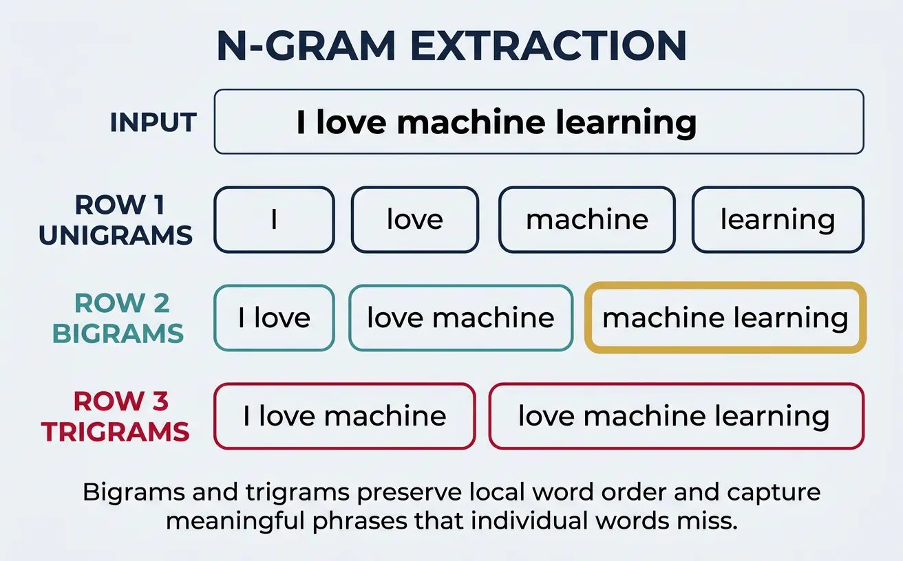
N-grams are contiguous sequences of N items (usually words or characters) from a text. While unigrams (single words) ignore word order, bigrams (2 words), trigrams (3 words), and higher-order n-grams capture local context and word co-occurrence patterns. This partial preservation of word order addresses a key limitation of simple BoW models.
For example, the sentence "I love machine learning" produces these n-grams: Unigrams: ["I", "love", "machine", "learning"]; Bigrams: ["I love", "love machine", "machine learning"]; Trigrams: ["I love machine", "love machine learning"]. Bigrams like "machine learning" capture meaningful phrases that individual words miss.
from sklearn.feature_extraction.text import CountVectorizer
import pandas as pd

text = "Natural language processing is a fascinating field of artificial intelligence"

# Generate different n-gram representations
unigram_vec = CountVectorizer(ngram_range=(1, 1))
bigram_vec = CountVectorizer(ngram_range=(2, 2))
trigram_vec = CountVectorizer(ngram_range=(3, 3))
combined_vec = CountVectorizer(ngram_range=(1, 3))

print("N-gram Analysis:")
print("=" * 60)

for name, vec in [("Unigrams (1,1)", unigram_vec),
                  ("Bigrams (2,2)", bigram_vec),
                  ("Trigrams (3,3)", trigram_vec),
                  ("Combined (1,3)", combined_vec)]:
    vec.fit([text])
    features = vec.get_feature_names_out()
    print(f"\n{name} - {len(features)} features:")
    print(", ".join(features[:10]))
    if len(features) > 10:
        print(f"  ... and {len(features) - 10} more")
Character vs Word N-grams
Character n-grams are useful for handling typos, morphological variations, and languages without clear word boundaries. Word n-grams capture phrases and collocations. Many modern systems use both for robust text representation.
from sklearn.feature_extraction.text import CountVectorizer

text = "The quick brown fox jumps"

# Character-level n-grams
char_vec = CountVectorizer(analyzer='char', ngram_range=(2, 4))
char_vec.fit([text])
char_ngrams = char_vec.get_feature_names_out()

print("Character N-grams (2-4):")
print("Sample:", list(char_ngrams[:15]))
print(f"Total: {len(char_ngrams)} features")

# Character n-grams within word boundaries (avoids cross-word n-grams)
char_wb_vec = CountVectorizer(analyzer='char_wb', ngram_range=(2, 4))
char_wb_vec.fit([text])
char_wb_ngrams = char_wb_vec.get_feature_names_out()

print("\nCharacter N-grams (word boundaries):")
print("Sample:", list(char_wb_ngrams[:15]))
print(f"Total: {len(char_wb_ngrams)} features")

# Practical example: handling typos
words = ["machine", "machne", "machin", "learning", "leanring"]
char_vec_typo = CountVectorizer(analyzer='char', ngram_range=(3, 3))
char_matrix = char_vec_typo.fit_transform(words)

from sklearn.metrics.pairwise import cosine_similarity
similarity = cosine_similarity(char_matrix)

print("\nTypo Similarity (character trigrams):")
for i, w1 in enumerate(words):
    for j, w2 in enumerate(words):
        if i < j:
            print(f"  '{w1}' vs '{w2}': {similarity[i,j]:.3f}")
N-gram Frequency Analysis
from sklearn.feature_extraction.text import CountVectorizer
import numpy as np

# Sample corpus
corpus = [
    "machine learning is transforming artificial intelligence research",
    "deep learning neural networks achieve state of the art results",
    "natural language processing uses machine learning models",
    "computer vision and machine learning work together",
    "artificial intelligence includes machine learning and deep learning"
]

# Extract bigrams
bigram_vec = CountVectorizer(ngram_range=(2, 2), stop_words='english')
bigram_matrix = bigram_vec.fit_transform(corpus)
bigram_features = bigram_vec.get_feature_names_out()

# Sum frequencies across documents
bigram_freq = np.array(bigram_matrix.sum(axis=0)).flatten()

# Sort by frequency
sorted_indices = bigram_freq.argsort()[::-1]

print("Most Common Bigrams in Corpus:")
print("-" * 40)
for i in sorted_indices[:10]:
    print(f"  '{bigram_features[i]}': {bigram_freq[i]:.0f} occurrences")

# Extract trigrams
trigram_vec = CountVectorizer(ngram_range=(3, 3), stop_words='english')
trigram_matrix = trigram_vec.fit_transform(corpus)
trigram_features = trigram_vec.get_feature_names_out()
trigram_freq = np.array(trigram_matrix.sum(axis=0)).flatten()
sorted_tri = trigram_freq.argsort()[::-1]

print("\nMost Common Trigrams:")
print("-" * 40)
for i in sorted_tri[:5]:
    if trigram_freq[i] > 0:
        print(f"  '{trigram_features[i]}': {trigram_freq[i]:.0f}")
Feature Engineering for NLP
Feature engineering in NLP goes beyond simple word representations to capture linguistic, structural, and domain-specific signals. While modern deep learning can learn features automatically, hand-crafted features remain valuable for improving model interpretability, reducing training data requirements, and combining with neural approaches in hybrid systems.
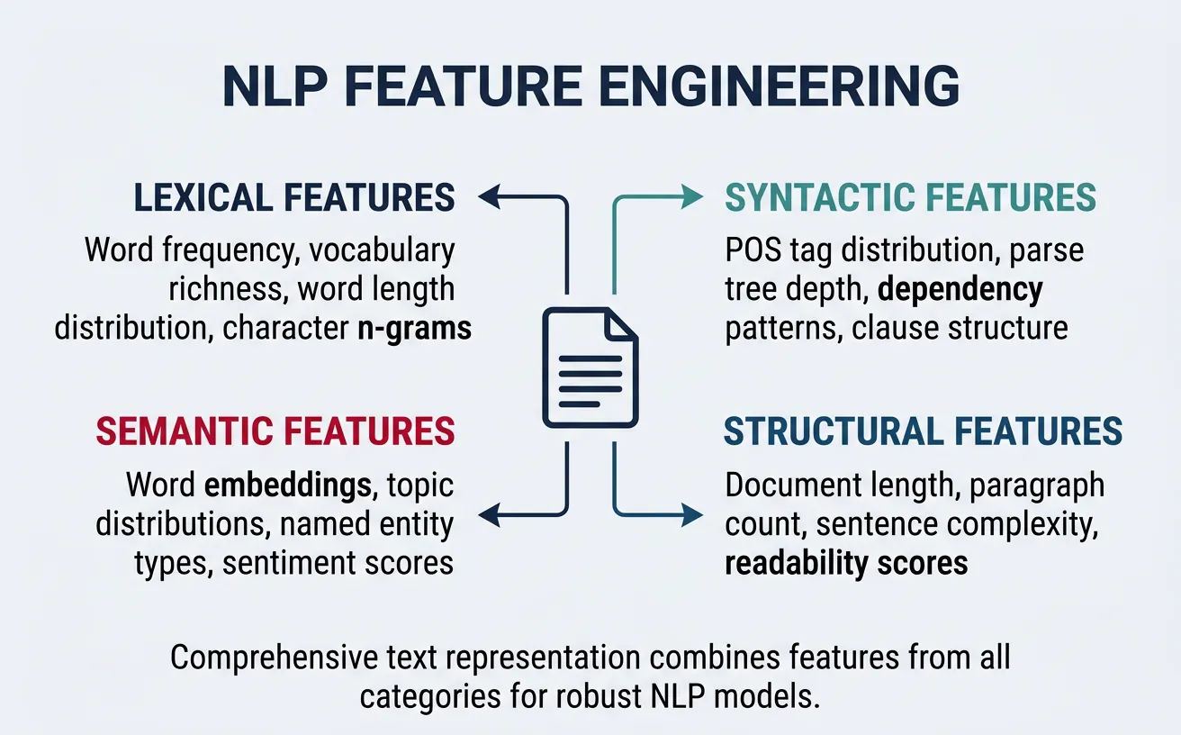
Effective NLP features fall into several categories: lexical features (word counts, vocabulary richness), syntactic features (POS tag distributions, parse tree depth), semantic features (named entities, sentiment words), and structural features (sentence length, punctuation patterns). The right feature set depends heavily on your task and domain.
import numpy as np
import re
from collections import Counter

def extract_text_features(text):
    """Extract comprehensive features from text."""
    words = text.split()
    sentences = re.split(r'[.!?]+', text)
    sentences = [s.strip() for s in sentences if s.strip()]

    features = {}

    # Basic statistics
    features['char_count'] = len(text)
    features['word_count'] = len(words)
    features['sentence_count'] = len(sentences)
    features['avg_word_length'] = np.mean([len(w) for w in words]) if words else 0
    features['avg_sentence_length'] = len(words) / len(sentences) if sentences else 0

    # Vocabulary richness
    unique_words = set(w.lower() for w in words)
    features['unique_word_count'] = len(unique_words)
    features['lexical_diversity'] = len(unique_words) / len(words) if words else 0

    # Punctuation features
    features['exclamation_count'] = text.count('!')
    features['question_count'] = text.count('?')
    features['comma_count'] = text.count(',')

    # Case features
    features['uppercase_ratio'] = sum(1 for c in text if c.isupper()) / len(text) if text else 0
    features['title_case_words'] = sum(1 for w in words if w.istitle())

    # Special patterns
    features['digit_count'] = sum(1 for c in text if c.isdigit())
    features['has_url'] = 1 if re.search(r'http[s]?://', text) else 0
    features['has_email'] = 1 if re.search(r'\S+@\S+', text) else 0

    return features

# Test on sample texts
texts = [
    "Machine learning is AMAZING! It's transforming every industry.",
    "The quick brown fox jumps over the lazy dog. Simple and short.",
    "Contact us at info@example.com or visit https://example.com for more info!"
]

print("Feature Extraction Results:")
print("=" * 70)
for i, text in enumerate(texts, 1):
    print(f"\nText {i}: '{text[:50]}...'")
    features = extract_text_features(text)
    for key, value in list(features.items())[:8]:
        print(f"  {key}: {value:.3f}" if isinstance(value, float) else f"  {key}: {value}")
Combining Features for Classification
from sklearn.feature_extraction.text import TfidfVectorizer
from sklearn.preprocessing import StandardScaler
from sklearn.pipeline import Pipeline, FeatureUnion
from sklearn.base import BaseEstimator, TransformerMixin
import numpy as np

class TextStatisticsExtractor(BaseEstimator, TransformerMixin):
    """Extract statistical features from text."""

    def fit(self, X, y=None):
        return self

    def transform(self, X):
        features = []
        for text in X:
            words = text.split()
            features.append([
                len(words),  # word count
                len(text),   # char count
                np.mean([len(w) for w in words]) if words else 0,  # avg word length
                len(set(words)) / len(words) if words else 0,  # lexical diversity
                sum(1 for c in text if c.isupper()) / len(text) if text else 0  # uppercase ratio
            ])
        return np.array(features)

# Create combined feature pipeline
combined_features = FeatureUnion([
    ('tfidf', TfidfVectorizer(max_features=100, stop_words='english')),
    ('stats', Pipeline([
        ('extract', TextStatisticsExtractor()),
        ('scale', StandardScaler())
    ]))
])

# Sample data
texts = [
    "Machine learning is revolutionizing data science!",
    "Simple text with few words.",
    "URGENT: This is a very important message with CAPITAL letters!"
]

# Transform
combined_matrix = combined_features.fit_transform(texts)
print(f"Combined feature shape: {combined_matrix.shape}")
print(f"  - TF-IDF features: 100")
print(f"  - Statistical features: 5")
print(f"  - Total: {combined_matrix.shape[1]}")
Sparse vs Dense Representations
Sparse representations (BoW, TF-IDF) have most values as zero because each document only contains a tiny fraction of the total vocabulary. A 50,000-word vocabulary means 50,000-dimensional vectors, but a typical document might only have 100-500 unique words. Dense representations (word embeddings, neural encodings) compress meaning into lower-dimensional vectors (typically 100-1000 dimensions) where most values are non-zero.
The choice between sparse and dense depends on your task, data size, and computational constraints. Sparse representations are interpretable and require no training but scale poorly. Dense representations capture semantic relationships and generalize better but require substantial training data and are less interpretable.
import numpy as np
from sklearn.feature_extraction.text import TfidfVectorizer
from scipy import sparse

# Sample corpus
corpus = [
    "Machine learning is a subset of artificial intelligence",
    "Deep learning uses neural networks for complex patterns",
    "Natural language processing analyzes human language"
]

# Create sparse TF-IDF matrix
vectorizer = TfidfVectorizer()
sparse_matrix = vectorizer.fit_transform(corpus)

print("Sparse Representation Analysis")
print("=" * 50)
print(f"Matrix shape: {sparse_matrix.shape}")
print(f"Data type: {type(sparse_matrix)}")
print(f"Storage format: {sparse_matrix.format}")

# Analyze sparsity
total_elements = sparse_matrix.shape[0] * sparse_matrix.shape[1]
non_zero = sparse_matrix.nnz
sparsity = (total_elements - non_zero) / total_elements * 100

print(f"\nSparsity Statistics:")
print(f"  Total elements: {total_elements}")
print(f"  Non-zero elements: {non_zero}")
print(f"  Sparsity: {sparsity:.1f}%")

# Memory comparison
dense_matrix = sparse_matrix.toarray()
sparse_memory = sparse_matrix.data.nbytes + sparse_matrix.indices.nbytes + sparse_matrix.indptr.nbytes
dense_memory = dense_matrix.nbytes

print(f"\nMemory Usage:")
print(f"  Sparse format: {sparse_memory:,} bytes")
print(f"  Dense format: {dense_memory:,} bytes")
print(f"  Compression ratio: {dense_memory / sparse_memory:.1f}x")
Sparse vs Dense: When to Use Each
| Aspect | Sparse (BoW/TF-IDF) | Dense (Embeddings) |
|---|---|---|
| Dimensionality | High (vocabulary size) | Low (100-1000) |
| Semantics | No semantic similarity | Captures meaning |
| Training | No training needed | Requires large corpus |
| Interpretability | High (direct word mapping) | Low (abstract dimensions) |
| OOV handling | Poor (unknown = zero) | Subword methods help |
| Best for | Search, classification baseline | Semantic tasks, deep learning |
Dimensionality Reduction for Sparse Vectors
from sklearn.feature_extraction.text import TfidfVectorizer
from sklearn.decomposition import TruncatedSVD
import numpy as np

# Larger corpus for meaningful dimensionality reduction
corpus = [
    "Machine learning algorithms learn patterns from data",
    "Deep learning is a type of machine learning",
    "Neural networks power deep learning systems",
    "Natural language processing analyzes text",
    "Computer vision processes images and videos",
    "Reinforcement learning uses rewards and penalties",
    "Supervised learning requires labeled training data",
    "Unsupervised learning finds hidden patterns",
    "Data science combines statistics and programming",
    "Artificial intelligence mimics human intelligence"
]

# Create TF-IDF matrix
vectorizer = TfidfVectorizer(stop_words='english')
tfidf_matrix = vectorizer.fit_transform(corpus)

print(f"Original TF-IDF shape: {tfidf_matrix.shape}")

# Apply Truncated SVD (LSA - Latent Semantic Analysis)
n_components = 5
svd = TruncatedSVD(n_components=n_components, random_state=42)
dense_matrix = svd.fit_transform(tfidf_matrix)

print(f"Reduced LSA shape: {dense_matrix.shape}")
print(f"Explained variance ratio: {svd.explained_variance_ratio_.sum():.2%}")

# Compare similarities in both spaces
from sklearn.metrics.pairwise import cosine_similarity

sparse_sim = cosine_similarity(tfidf_matrix[0:1], tfidf_matrix)
dense_sim = cosine_similarity(dense_matrix[0:1], dense_matrix)

print("\nSimilarity to Document 0:")
print(f"{'Document':<12} {'Sparse':<10} {'Dense':<10}")
print("-" * 32)
for i in range(min(5, len(corpus))):
    print(f"Doc {i:<8} {sparse_sim[0,i]:<10.3f} {dense_sim[0,i]:<10.3f}")
Conclusion & Next Steps
Text representation is the bridge between human language and machine learning algorithms. We've explored the progression from simple one-hot encoding to Bag of Words, then to TF-IDF weighting that accounts for term importance, and finally to N-grams that capture local word context. Each method has its place: one-hot for categorical encoding, BoW for baselines, TF-IDF for search and classification, and N-grams for phrase-aware applications.
Feature engineering extends these representations with hand-crafted signals that capture linguistic and domain-specific patterns. While deep learning has reduced the need for manual feature design, combining classical features with neural approaches often yields the best results. Understanding when to use sparse vs dense representations helps you make informed decisions about model architecture and computational trade-offs.
Key Takeaways
- One-Hot Encoding: Simple but doesn't scale; foundation for understanding other methods
- Bag of Words: Effective baseline that ignores word order but captures term frequency
- TF-IDF: Weights terms by importance; excellent for search and classification
- N-grams: Preserves local word context; captures meaningful phrases
- Feature Engineering: Domain knowledge encoded as numerical features
- Sparse vs Dense: Choose based on interpretability, semantics, and scale requirements
In Part 4: Word Embeddings, we'll move beyond sparse, count-based representations to dense vectors that capture semantic meaning. You'll learn how Word2Vec, GloVe, and FastText learn to represent words in continuous vector spaces where similar words have similar vectors—enabling mathematical operations on meaning itself.
Practice Exercises
- Document Classifier: Build a TF-IDF + Naive Bayes classifier for the 20 Newsgroups dataset
- Search Engine: Create a simple search engine using TF-IDF cosine similarity
- N-gram Analysis: Extract the most common bigrams and trigrams from a book corpus
- Feature Comparison: Compare classification accuracy with BoW, TF-IDF, and TF-IDF + statistical features
- LSA Exploration: Apply TruncatedSVD to TF-IDF and visualize document clusters in 2D