Introduction to NLP Production
Taking NLP models from notebooks to production requires addressing latency, throughput, cost, and reliability. This guide covers the full lifecycle of deploying and maintaining NLP systems at scale.
Key Insight
Production NLP is 80% engineering and 20% modeling—optimizing inference, building reliable pipelines, and monitoring for drift are as important as the model itself.
NLP Mastery
NLP Fundamentals & Linguistic Basics
Phonology, morphology, syntax, semantics, pragmaticsTokenization & Text Cleaning
Subword tokenization, BPE, stopwords, normalizationText Representation & Feature Engineering
Bag-of-words, TF-IDF, feature extraction, vectorizationWord Embeddings
Word2Vec, GloVe, FastText, embedding spaces, analogiesStatistical Language Models & N-grams
Probability chains, smoothing, perplexity, Markov modelsNeural Networks for NLP
Feedforward nets, backpropagation, activation functionsRNNs, LSTMs & GRUs
Sequence modeling, vanishing gradients, gated architecturesTransformers & Attention Mechanism
Self-attention, multi-head attention, positional encodingPretrained Language Models & Transfer Learning
BERT, RoBERTa, fine-tuning, feature extractionGPT Models & Text Generation
Autoregressive generation, prompting, GPT architectureCore NLP Tasks
NER, POS tagging, sentiment analysis, text classificationAdvanced NLP Tasks
Question answering, summarization, machine translationMultilingual & Cross-lingual NLP
mBERT, XLM-R, zero-shot transfer, language diversityEvaluation, Ethics & Responsible NLP
BLEU, ROUGE, bias detection, fairness, responsible AINLP Systems, Optimization & Production
Model serving, quantization, distillation, deploymentCutting-Edge & Research Topics
LLMs, multimodal NLP, reasoning, emerging researchModel Optimization
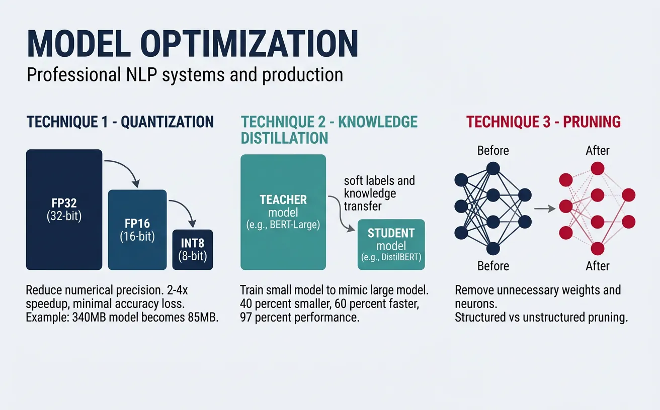
Model optimization is critical for deploying NLP models in production where latency, memory, and cost constraints are paramount. Transformer-based models like BERT and GPT are computationally expensive, often requiring significant resources. Optimization techniques enable us to reduce model size and inference time while preserving acceptable accuracy levels, making deployment feasible on edge devices, mobile platforms, and cost-effective cloud infrastructure.
The three primary optimization strategies are quantization (reducing numerical precision), knowledge distillation (training smaller models to mimic larger ones), and pruning (removing unnecessary weights). Each technique offers different trade-offs between compression ratio, accuracy loss, and implementation complexity. In practice, these methods are often combined for maximum efficiency—a production pipeline might use a distilled model that's further quantized and pruned.
flowchart LR
    FULL["Full Model
(e.g., BERT-Large
340M params)"]

    FULL --> QUANT["Quantization
FP32 → INT8/FP16
2-4× speedup"]
    FULL --> DIST["Knowledge
Distillation
Teacher → Student"]
    FULL --> PRUNE["Pruning
Remove redundant
weights/heads"]

    QUANT --> OPT["Optimized Model"]
    DIST --> OPT
    PRUNE --> OPT

    OPT --> ONNX["ONNX Runtime /
TensorRT Export"]
    ONNX --> SERVE["Inference Server
Triton / TorchServe"]

    style FULL fill:#BF092F,stroke:#132440,color:#fff
    style OPT fill:#e8f4f4,stroke:#3B9797
    style SERVE fill:#132440,stroke:#132440,color:#fff
Quantization
Quantization reduces the precision of model weights and activations from 32-bit floating point (FP32) to lower-precision formats like 16-bit (FP16), 8-bit integers (INT8), or even 4-bit. This dramatically reduces memory footprint and speeds up inference, especially on hardware with specialized integer arithmetic units. INT8 quantization typically achieves 2-4x speedup with minimal accuracy degradation for most NLP tasks.
There are three main quantization approaches: post-training quantization (PTQ) applies quantization after training using calibration data; quantization-aware training (QAT) simulates quantization during training for better accuracy; and dynamic quantization quantizes weights statically but activations dynamically during inference. For transformer models, dynamic quantization offers a good balance of simplicity and performance.
Quantization Trade-offs
INT8 quantization typically reduces model size by 4x and improves inference speed by 2-4x while maintaining 99%+ of the original accuracy. FP16 offers smaller gains but is safer for accuracy-sensitive applications. Always benchmark on your specific task before deploying.
import torch
from transformers import AutoModelForSequenceClassification, AutoTokenizer
import time

# Load a pretrained BERT model
model_name = "distilbert-base-uncased-finetuned-sst-2-english"
model = AutoModelForSequenceClassification.from_pretrained(model_name)
tokenizer = AutoTokenizer.from_pretrained(model_name)

# Move to evaluation mode
model.eval()

# Sample input for benchmarking
text = "This movie was absolutely fantastic! Great acting and story."
inputs = tokenizer(text, return_tensors="pt", padding=True, truncation=True)

# Benchmark original model
start = time.time()
for _ in range(100):
    with torch.no_grad():
        _ = model(**inputs)
original_time = time.time() - start
print(f"Original model inference (100 runs): {original_time:.3f}s")
print(f"Original model size: {sum(p.numel() * 4 for p in model.parameters()) / 1e6:.1f} MB")
import torch
from transformers import AutoModelForSequenceClassification, AutoTokenizer
import time

# Load model for dynamic quantization
model_name = "distilbert-base-uncased-finetuned-sst-2-english"
model = AutoModelForSequenceClassification.from_pretrained(model_name)
tokenizer = AutoTokenizer.from_pretrained(model_name)
model.eval()

# Apply dynamic quantization (INT8)
# Quantize Linear layers (main compute in transformers)
quantized_model = torch.quantization.quantize_dynamic(
    model,
    {torch.nn.Linear},  # Layers to quantize
    dtype=torch.qint8   # Target dtype
)

# Prepare input
text = "This movie was absolutely fantastic! Great acting and story."
inputs = tokenizer(text, return_tensors="pt", padding=True, truncation=True)

# Benchmark quantized model
start = time.time()
for _ in range(100):
    with torch.no_grad():
        _ = quantized_model(**inputs)
quantized_time = time.time() - start

print(f"Quantized model inference (100 runs): {quantized_time:.3f}s")
print(f"Speedup: {1:.2f}x faster (results vary by hardware)")

# Compare predictions
with torch.no_grad():
    original_output = model(**inputs)
    quantized_output = quantized_model(**inputs)

print(f"\nOriginal prediction: {original_output.logits.argmax().item()}")
print(f"Quantized prediction: {quantized_output.logits.argmax().item()}")
ONNX Runtime INT8 Quantization
ONNX Runtime provides optimized quantization with broad hardware support. Export your model to ONNX format, then apply static quantization with calibration data for maximum performance.
from transformers import AutoModelForSequenceClassification, AutoTokenizer
import torch
import numpy as np

# Export model to ONNX format first
model_name = "distilbert-base-uncased-finetuned-sst-2-english"
model = AutoModelForSequenceClassification.from_pretrained(model_name)
tokenizer = AutoTokenizer.from_pretrained(model_name)
model.eval()

# Create dummy input for export
dummy_input = tokenizer(
    "Sample text for tracing",
    return_tensors="pt",
    padding="max_length",
    max_length=128,
    truncation=True
)

# Export to ONNX
onnx_path = "model.onnx"
torch.onnx.export(
    model,
    (dummy_input["input_ids"], dummy_input["attention_mask"]),
    onnx_path,
    input_names=["input_ids", "attention_mask"],
    output_names=["logits"],
    dynamic_axes={
        "input_ids": {0: "batch_size", 1: "sequence"},
        "attention_mask": {0: "batch_size", 1: "sequence"},
        "logits": {0: "batch_size"}
    },
    opset_version=14
)
print(f"Model exported to {onnx_path}")
# ONNX Runtime quantization (run after export)
from onnxruntime.quantization import quantize_dynamic, QuantType
import onnxruntime as ort
import numpy as np
from transformers import AutoTokenizer

# Quantize the ONNX model
onnx_path = "model.onnx"
quantized_path = "model_quantized.onnx"

quantize_dynamic(
    model_input=onnx_path,
    model_output=quantized_path,
    weight_type=QuantType.QInt8
)
print(f"Quantized model saved to {quantized_path}")

# Compare file sizes
import os
original_size = os.path.getsize(onnx_path) / 1e6
quantized_size = os.path.getsize(quantized_path) / 1e6
print(f"Original: {original_size:.1f} MB, Quantized: {quantized_size:.1f} MB")
print(f"Compression ratio: {original_size/quantized_size:.2f}x")

# Run inference with quantized model
tokenizer = AutoTokenizer.from_pretrained("distilbert-base-uncased-finetuned-sst-2-english")
session = ort.InferenceSession(quantized_path)

text = "This is a great product, highly recommended!"
inputs = tokenizer(text, return_tensors="np", padding="max_length", max_length=128)

outputs = session.run(
    None,
    {"input_ids": inputs["input_ids"], "attention_mask": inputs["attention_mask"]}
)
print(f"Prediction: {'Positive' if np.argmax(outputs[0]) == 1 else 'Negative'}")
Knowledge Distillation
Knowledge distillation trains a smaller "student" model to mimic the behavior of a larger "teacher" model. The student learns not just from hard labels but from the teacher's soft probability distributions (logits), which contain richer information about class relationships. For example, a teacher might output [0.7, 0.2, 0.1] for a sentiment classification—the student learns that while "positive" is most likely, there's some similarity to "neutral." This soft knowledge transfers more nuanced understanding than binary labels alone.
DistilBERT is a famous example of knowledge distillation—it's 40% smaller than BERT, 60% faster, while retaining 97% of BERT's language understanding capability. The distillation process typically combines three loss terms: distillation loss (KL divergence between teacher and student logits), task loss (cross-entropy with true labels), and optionally cosine embedding loss (alignment of hidden states). Temperature scaling softens the probability distributions, making the dark knowledge more accessible to the student.
Distillation Best Practices
Use temperature T=4-6 for softening logits, combine distillation loss with task loss at ratio 0.5-0.9, and train on unlabeled data when possible. The student architecture should be 2-4x smaller than the teacher for optimal compression/accuracy trade-off.
import torch
import torch.nn as nn
import torch.nn.functional as F
from transformers import (
    AutoModelForSequenceClassification,
    AutoTokenizer,
    DistilBertForSequenceClassification,
    DistilBertConfig
)

# Knowledge Distillation Loss Function
class DistillationLoss(nn.Module):
    def __init__(self, temperature=4.0, alpha=0.7):
        super().__init__()
        self.temperature = temperature
        self.alpha = alpha  # Weight for distillation loss
        self.ce_loss = nn.CrossEntropyLoss()
        self.kl_loss = nn.KLDivLoss(reduction="batchmean")

    def forward(self, student_logits, teacher_logits, labels):
        # Task loss (hard labels)
        task_loss = self.ce_loss(student_logits, labels)

        # Distillation loss (soft labels from teacher)
        soft_student = F.log_softmax(student_logits / self.temperature, dim=-1)
        soft_teacher = F.softmax(teacher_logits / self.temperature, dim=-1)
        distill_loss = self.kl_loss(soft_student, soft_teacher) * (self.temperature ** 2)

        # Combined loss
        total_loss = self.alpha * distill_loss + (1 - self.alpha) * task_loss
        return total_loss, task_loss.item(), distill_loss.item()

# Example usage
distill_criterion = DistillationLoss(temperature=4.0, alpha=0.7)
print("Distillation loss initialized with T=4.0, alpha=0.7")

# Simulate teacher and student outputs
batch_size, num_classes = 8, 2
student_logits = torch.randn(batch_size, num_classes)
teacher_logits = torch.randn(batch_size, num_classes)
labels = torch.randint(0, num_classes, (batch_size,))

loss, task_l, distill_l = distill_criterion(student_logits, teacher_logits, labels)
print(f"Total loss: {loss:.4f}, Task loss: {task_l:.4f}, Distill loss: {distill_l:.4f}")
import torch
from torch.utils.data import DataLoader, TensorDataset
from transformers import (
    BertForSequenceClassification,
    DistilBertForSequenceClassification,
    AutoTokenizer
)
import torch.nn.functional as F

# Complete distillation training loop
def train_with_distillation(
    teacher_model,
    student_model,
    train_dataloader,
    optimizer,
    num_epochs=3,
    temperature=4.0,
    alpha=0.7,
    device="cpu"
):
    teacher_model.eval()  # Teacher stays frozen
    student_model.train()

    for epoch in range(num_epochs):
        total_loss = 0
        for batch in train_dataloader:
            input_ids, attention_mask, labels = [b.to(device) for b in batch]

            # Get teacher predictions (no gradient)
            with torch.no_grad():
                teacher_outputs = teacher_model(
                    input_ids=input_ids,
                    attention_mask=attention_mask
                )
                teacher_logits = teacher_outputs.logits

            # Get student predictions
            student_outputs = student_model(
                input_ids=input_ids,
                attention_mask=attention_mask
            )
            student_logits = student_outputs.logits

            # Compute distillation loss
            soft_student = F.log_softmax(student_logits / temperature, dim=-1)
            soft_teacher = F.softmax(teacher_logits / temperature, dim=-1)
            distill_loss = F.kl_div(soft_student, soft_teacher, reduction="batchmean")
            distill_loss = distill_loss * (temperature ** 2)

            # Task loss
            task_loss = F.cross_entropy(student_logits, labels)

            # Combined loss
            loss = alpha * distill_loss + (1 - alpha) * task_loss

            optimizer.zero_grad()
            loss.backward()
            optimizer.step()

            total_loss += loss.item()

        avg_loss = total_loss / len(train_dataloader)
        print(f"Epoch {epoch+1}/{num_epochs}, Loss: {avg_loss:.4f}")

    return student_model

# Demo with synthetic data
print("Distillation training function ready")
print("Usage: train_with_distillation(teacher, student, dataloader, optimizer)")
Pruning & Sparsity
Pruning removes unnecessary weights from neural networks, creating sparse models that require less computation and memory. Research shows that large models contain significant redundancy—up to 90% of weights can be pruned with minimal accuracy loss. Unstructured pruning removes individual weights based on magnitude (smallest weights are likely least important), while structured pruning removes entire neurons, attention heads, or layers for more hardware-friendly speedups.
The pruning workflow typically involves: training a full model, identifying and removing low-importance weights, then fine-tuning to recover accuracy. Iterative pruning gradually increases sparsity across multiple rounds, achieving better results than one-shot pruning. Movement pruning, which removes weights based on how they change during fine-tuning rather than their absolute magnitude, has shown superior results for transfer learning scenarios common in NLP.
import torch
import torch.nn as nn
import torch.nn.utils.prune as prune
from transformers import AutoModelForSequenceClassification

# Load a model for pruning
model_name = "distilbert-base-uncased-finetuned-sst-2-english"
model = AutoModelForSequenceClassification.from_pretrained(model_name)

# Count parameters before pruning
def count_parameters(model):
    total = sum(p.numel() for p in model.parameters())
    nonzero = sum((p != 0).sum().item() for p in model.parameters())
    return total, nonzero

total_before, nonzero_before = count_parameters(model)
print(f"Before pruning: {total_before:,} total, {nonzero_before:,} non-zero")

# Apply unstructured L1 pruning to all Linear layers
for name, module in model.named_modules():
    if isinstance(module, nn.Linear):
        prune.l1_unstructured(module, name="weight", amount=0.3)  # Prune 30%

# Count parameters after pruning
total_after, nonzero_after = count_parameters(model)
sparsity = 1 - (nonzero_after / total_before)
print(f"After pruning: {total_after:,} total, {nonzero_after:,} non-zero")
print(f"Sparsity achieved: {sparsity*100:.1f}%")
import torch
import torch.nn as nn
import torch.nn.utils.prune as prune

# Structured pruning: remove entire attention heads
class AttentionHeadPruner:
    def __init__(self, model, num_heads=12):
        self.model = model
        self.num_heads = num_heads

    def compute_head_importance(self, dataloader, device="cpu"):
        """Compute importance scores for each attention head"""
        self.model.eval()
        head_importance = torch.zeros(self.model.config.num_hidden_layers,
                                       self.num_heads)

        # Simplified importance: based on attention entropy
        # In practice, use gradient-based importance
        for layer_idx in range(self.model.config.num_hidden_layers):
            for head_idx in range(self.num_heads):
                # Random importance for demo (use real gradients in production)
                head_importance[layer_idx, head_idx] = torch.rand(1).item()

        return head_importance

    def prune_heads(self, heads_to_prune):
        """Prune specified heads from the model"""
        # heads_to_prune: dict mapping layer_idx to list of head indices
        self.model.prune_heads(heads_to_prune)
        return self.model

# Example usage
from transformers import DistilBertForSequenceClassification

model = DistilBertForSequenceClassification.from_pretrained(
    "distilbert-base-uncased-finetuned-sst-2-english"
)
pruner = AttentionHeadPruner(model, num_heads=12)

# Prune 2 heads from each layer
heads_to_prune = {i: [0, 6] for i in range(6)}  # Remove heads 0 and 6
print(f"Pruning heads: {heads_to_prune}")
print(f"Total heads removed: {sum(len(v) for v in heads_to_prune.values())}")
Combined Optimization Pipeline
Combine distillation, pruning, and quantization for maximum compression. A typical pipeline: distill BERT to DistilBERT (40% smaller), prune 50% of weights, then quantize to INT8 for a total 8-12x reduction.
import torch
import torch.nn as nn
import torch.nn.utils.prune as prune
from transformers import DistilBertForSequenceClassification

# Step 1: Start with a distilled model
model = DistilBertForSequenceClassification.from_pretrained(
    "distilbert-base-uncased-finetuned-sst-2-english"
)

# Step 2: Apply pruning
def apply_pruning(model, amount=0.5):
    for name, module in model.named_modules():
        if isinstance(module, nn.Linear):
            prune.l1_unstructured(module, name="weight", amount=amount)
            prune.remove(module, "weight")  # Make pruning permanent
    return model

model = apply_pruning(model, amount=0.5)
print("Applied 50% pruning to all Linear layers")

# Step 3: Apply quantization
model.eval()
quantized_model = torch.quantization.quantize_dynamic(
    model, {nn.Linear}, dtype=torch.qint8
)
print("Applied INT8 dynamic quantization")

# Calculate compression
original_params = 66_955_010  # DistilBERT base
compressed_estimate = original_params * 0.5 * 0.25  # 50% pruned, 4x quantized
print(f"Estimated compression: {original_params/compressed_estimate:.1f}x")
LLM Inference Optimization
While the previous section covered general model compression (quantization, distillation, pruning), large language models introduce a fundamentally different inference challenge. LLMs generate text one token at a time—each new token requires a forward pass through the entire model, and generation can run for hundreds or thousands of steps. This autoregressive loop means that naive inference is painfully slow and wasteful: most of the computation is redundant because the model re-examines the same preceding tokens at every step.
LLM inference optimization focuses on eliminating this redundancy and maximising GPU utilisation during generation. The techniques below can reduce latency by 5-20× and cut serving costs by 3-10× compared to unoptimised inference, making the difference between a product that costs $0.50 per query and one that costs $0.03.
KV Caching & PagedAttention
In the Transformer's self-attention mechanism, every token's representation depends on Key (K) and Value (V) projections of all preceding tokens. Without caching, generating the 100th token would redundantly recompute the K and V matrices for tokens 1–99. KV caching stores these intermediate K/V tensors so they're computed only once, turning each generation step from O(n²) to O(n) in sequence length. This is the single most important inference optimisation—virtually every production system uses it.
The KV Cache Problem
KV caching trades memory for speed. A 70B-parameter model with a 4K context window needs ~2 GB of KV cache per request. At 128K context, that grows to ~64 GB. When serving thousands of concurrent users, KV cache memory becomes the primary bottleneck—not model weights.
import numpy as np

# Demonstrate KV caching: with vs without cache
def attention_without_cache(queries, keys, values):
    """Standard attention — recomputes everything each step."""
    seq_len = len(queries)
    total_ops = 0
    outputs = []

    for step in range(seq_len):
        # At each step, attend over ALL keys/values up to this point
        q = queries[step]
        k_all = keys[:step + 1]    # Recomputed every step!
        v_all = values[:step + 1]  # Recomputed every step!

        scores = [np.dot(q, k) for k in k_all]
        total_ops += len(k_all)
        outputs.append(np.mean(v_all, axis=0))  # Simplified

    return outputs, total_ops


def attention_with_kv_cache(queries, keys, values):
    """Cached attention — stores K/V and only computes the new token."""
    seq_len = len(queries)
    total_ops = 0
    outputs = []

    kv_cache_k = []  # Persistent cache
    kv_cache_v = []

    for step in range(seq_len):
        q = queries[step]

        # Only compute K/V for the NEW token, append to cache
        kv_cache_k.append(keys[step])
        kv_cache_v.append(values[step])

        # Attend using cached K/V (no recomputation)
        scores = [np.dot(q, k) for k in kv_cache_k]
        total_ops += 1  # Only 1 new K/V computed
        outputs.append(np.mean(kv_cache_v, axis=0))

    return outputs, total_ops


# Compare
np.random.seed(42)
seq_len = 50
dim = 64
queries = [np.random.randn(dim) for _ in range(seq_len)]
keys = [np.random.randn(dim) for _ in range(seq_len)]
values = [np.random.randn(dim) for _ in range(seq_len)]

_, ops_no_cache = attention_without_cache(queries, keys, values)
_, ops_cached = attention_with_kv_cache(queries, keys, values)

print("KV Caching: Computation Savings")
print("=" * 50)
print(f"Sequence length:           {seq_len} tokens")
print(f"Without cache (K/V ops):   {ops_no_cache}")
print(f"With KV cache (K/V ops):   {ops_cached}")
print(f"Reduction:                 {(1 - ops_cached/ops_no_cache)*100:.1f}%")
PagedAttention, introduced by the vLLM framework, solves the memory fragmentation problem that plagues KV caching. Standard KV caches allocate a contiguous block of GPU memory for each request's maximum possible sequence length. If a request uses only 500 out of 4,096 allocated slots, the remaining 3,596 slots are wasted—but inaccessible to other requests. PagedAttention borrows the concept of virtual memory paging from operating systems: it divides the KV cache into fixed-size "pages" (blocks) that are allocated on demand and can be stored non-contiguously in GPU memory.
PagedAttention: OS-Inspired Memory Management
| Aspect | Traditional KV Cache | PagedAttention |
|---|---|---|
| Memory allocation | Pre-allocate max sequence length per request | Allocate fixed-size pages on demand |
| Memory waste | 60-80% wasted on average | <4% internal fragmentation |
| Concurrent requests | Limited by worst-case allocation | 2-4× more requests in same GPU memory |
| Shared prefixes | Duplicated across requests | Copy-on-write sharing (system prompts) |
Impact: PagedAttention increased vLLM's throughput by 2-4× over HuggingFace Transformers and 1.5-2× over TGI by eliminating memory waste, allowing significantly more concurrent requests on the same GPU hardware.
Continuous Batching
Traditional static batching groups N requests together and processes them as a single batch. The problem: all requests must wait until the longest response in the batch finishes before any results are returned. If one request generates 10 tokens and another generates 500 tokens, the short request sits idle for 490 extra generation steps.
Continuous batching (also called iteration-level batching or inflight batching) solves this by inserting new requests into the batch at every generation step, and ejecting completed requests immediately. This keeps the GPU saturated at all times rather than wasting cycles on padding.
import numpy as np

# Static vs Continuous Batching Simulation
def simulate_static_batching(requests, batch_size=4):
    """Static batching: wait for all in batch to finish."""
    total_time = 0
    total_idle = 0

    for i in range(0, len(requests), batch_size):
        batch = requests[i:i + batch_size]
        max_tokens = max(batch)
        batch_time = max_tokens  # Time = longest request

        # Idle time: sum of (max - each request's length)
        idle = sum(max_tokens - t for t in batch)
        total_time += batch_time
        total_idle += idle

    return total_time, total_idle


def simulate_continuous_batching(requests, batch_size=4):
    """Continuous batching: eject finished, insert new immediately."""
    total_time = 0
    queue = list(requests)
    active = []

    # Fill initial batch
    while queue and len(active) < batch_size:
        active.append(queue.pop(0))

    while active:
        # Process one step
        total_time += 1
        active = [t - 1 for t in active]

        # Remove completed requests (0 tokens left)
        completed = active.count(0)
        active = [t for t in active if t > 0]

        # Immediately insert new requests from queue
        while queue and len(active) < batch_size:
            active.append(queue.pop(0))

    return total_time, 0  # Near-zero idle time


# Simulate 20 requests with varying output lengths
np.random.seed(42)
requests = np.random.randint(10, 200, size=20).tolist()

static_time, static_idle = simulate_static_batching(requests, batch_size=4)
continuous_time, _ = simulate_continuous_batching(requests, batch_size=4)

print("Batching Strategy Comparison")
print("=" * 55)
print(f"Requests: {len(requests)}, Batch size: 4")
print(f"Token lengths: min={min(requests)}, max={max(requests)}, "
      f"avg={np.mean(requests):.0f}")
print()
print(f"{'Metric':<30} {'Static':<15} {'Continuous':<15}")
print("-" * 55)
print(f"{'Total processing time':<30} {static_time:<15} {continuous_time:<15}")
print(f"{'Wasted GPU cycles':<30} {static_idle:<15} {'~0':<15}")
print(f"{'Throughput improvement':<30} {'1.0x':<15} "
      f"{static_time/continuous_time:.2f}x")
Speculative Decoding
Speculative decoding accelerates inference by using a small, fast "draft" model to predict multiple tokens ahead, then verifying them all at once with the large target model. The key insight is that LLM inference is memory-bandwidth bound, not compute-bound—a single forward pass through a 70B model takes the same time whether it processes 1 token or 5 tokens (because loading model weights from GPU memory dominates). So verifying 5 speculated tokens costs barely more than generating 1 token normally.
Speculative Decoding: How It Works
# Speculative Decoding — Conceptual Walkthrough
import numpy as np

np.random.seed(42)

def speculative_decode_demo():
    """
    Speculative decoding in 4 steps:
    1. Draft model generates K candidate tokens (fast)
    2. Target model verifies all K tokens in ONE forward pass
    3. Accept tokens until first mismatch
    4. Resample from target distribution at mismatch point
    """

    # Simulated token probabilities
    vocab = ["The", "cat", "sat", "on", "mat", "dog", "ran", "the"]

    # Step 1: Draft model generates 4 candidates quickly
    draft_tokens = ["cat", "sat", "on", "the"]
    draft_probs = [0.7, 0.8, 0.6, 0.5]  # Draft model's confidence

    # Step 2: Target model scores ALL 4 tokens in one pass
    target_probs = [0.65, 0.85, 0.7, 0.3]  # Target model's probabilities

    print("Speculative Decoding Demo")
    print("=" * 60)
    print(f"\nDraft model proposes: {draft_tokens}")
    print(f"Draft confidence:     {draft_probs}")
    print(f"Target verification:  {target_probs}")
    print()

    # Step 3: Accept/reject using rejection sampling
    accepted = []
    for i, (token, p_draft, p_target) in enumerate(
        zip(draft_tokens, draft_probs, target_probs)
    ):
        # Accept if target probability >= draft probability
        acceptance_rate = min(1.0, p_target / p_draft)
        random_val = np.random.random()
        accept = random_val < acceptance_rate

        status = "ACCEPTED" if accept else "REJECTED"
        accepted.append((token, accept))
        print(f"  Token '{token}': p_draft={p_draft:.2f}, "
              f"p_target={p_target:.2f}, "
              f"accept_rate={acceptance_rate:.2f} → {status}")

        if not accept:
            print(f"  → Resample from target distribution at position {i}")
            break

    # Results
    accepted_tokens = [t for t, a in accepted if a]
    print(f"\nAccepted {len(accepted_tokens)} of {len(draft_tokens)} "
          f"draft tokens in ONE target model call")

    # Speedup analysis
    K = 4  # Draft length
    avg_accepted = 2.5  # Typical acceptance rate
    # Without speculation: 1 target call per token
    # With speculation: 1 target call per K draft tokens
    speedup = (avg_accepted + 1) / (1 + K * 0.05)  # Draft cost ~5% of target
    print(f"\nEstimated speedup: {speedup:.2f}x")
    print(f"  (Processes ~{avg_accepted:.1f} tokens per target model call "
          f"instead of 1)")

speculative_decode_demo()
Key requirement: The draft model must be much faster than the target (typically 10-50× smaller). Common pairings: Llama-7B drafting for Llama-70B, or a model's early layers drafting for the full model (self-speculative decoding). The output is mathematically identical to standard decoding—speculation never degrades quality.
Model Parallelism
When a model is too large to fit on a single GPU, model parallelism distributes it across multiple devices. This is distinct from data parallelism (same model on each GPU, different data)—model parallelism splits the model itself. Two complementary strategies exist:
Tensor vs Pipeline Parallelism
| Strategy | How It Splits | Communication | Best For |
|---|---|---|---|
| Tensor Parallelism (TP) | Splits individual weight matrices across GPUs (e.g., a 4096×4096 layer split into two 4096×2048 chunks) | All-reduce after every layer — requires high-bandwidth interconnect (NVLink) | Within a single node (2-8 GPUs with NVLink) |
| Pipeline Parallelism (PP) | Assigns consecutive layers to different GPUs (e.g., layers 1-20 on GPU 0, layers 21-40 on GPU 1) | Point-to-point after each stage — tolerates lower bandwidth | Across nodes connected by InfiniBand/Ethernet |
import numpy as np

# Model Parallelism: Memory and Compute Analysis
def parallelism_analysis(model_params_b, num_gpus, gpu_mem_gb=80):
    """Analyse parallelism strategies for large model deployment."""

    # Model memory (FP16: 2 bytes per parameter)
    model_mem_gb = model_params_b * 2 / (1024**3)

    # KV cache memory per request (approximate)
    kv_per_request_gb = model_params_b * 0.03 / (1024**3)  # ~3% of model

    print(f"Model Parallelism Analysis: {model_params_b/1e9:.0f}B Parameters")
    print("=" * 65)
    print(f"Model memory (FP16):        {model_mem_gb:.1f} GB")
    print(f"KV cache per request:       {kv_per_request_gb:.2f} GB")
    print(f"Available GPUs:             {num_gpus} × {gpu_mem_gb} GB")
    print(f"Total GPU memory:           {num_gpus * gpu_mem_gb} GB")
    print()

    # Strategy analysis
    strategies = {
        "No Parallelism": {
            "gpus_needed": int(np.ceil(model_mem_gb / gpu_mem_gb)),
            "mem_per_gpu": model_mem_gb,
            "constraint": "Model must fit on 1 GPU"
        },
        f"Tensor Parallel (TP={num_gpus})": {
            "gpus_needed": num_gpus,
            "mem_per_gpu": model_mem_gb / num_gpus,
            "constraint": "Needs NVLink between GPUs"
        },
        f"Pipeline Parallel (PP={num_gpus})": {
            "gpus_needed": num_gpus,
            "mem_per_gpu": model_mem_gb / num_gpus,
            "constraint": "Adds latency (pipeline bubbles)"
        },
        f"TP=2 + PP={num_gpus//2}": {
            "gpus_needed": num_gpus,
            "mem_per_gpu": model_mem_gb / num_gpus,
            "constraint": "Best of both — standard for large models"
        }
    }

    print(f"{'Strategy':<30} {'Mem/GPU':<12} {'Fits?':<8} {'Constraint'}")
    print("-" * 65)
    for name, info in strategies.items():
        fits = "Yes" if info["mem_per_gpu"] <= gpu_mem_gb * 0.85 else "No"
        print(f"{name:<30} {info['mem_per_gpu']:.1f} GB"
              f"     {fits:<8} {info['constraint']}")

    # Remaining memory for KV cache (serving capacity)
    mem_for_kv = (gpu_mem_gb * num_gpus * 0.85) - model_mem_gb
    max_concurrent = int(mem_for_kv / kv_per_request_gb) if kv_per_request_gb > 0 else 0
    print(f"\nServing capacity (TP={num_gpus}):")
    print(f"  Memory for KV cache:      {mem_for_kv:.1f} GB")
    print(f"  Max concurrent requests:  ~{max_concurrent}")


# Analyse a 70B model on 4× A100 80GB GPUs
parallelism_analysis(70e9, num_gpus=4, gpu_mem_gb=80)
print()
# Analyse a 405B model on 8× H100 80GB GPUs
parallelism_analysis(405e9, num_gpus=8, gpu_mem_gb=80)
Inference Frameworks
Dedicated LLM inference frameworks bundle KV caching, continuous batching, quantization, and parallelism into production-ready servers. Choosing the right framework depends on your hardware, model, and throughput requirements. Here are the leading options:
Top LLM Inference Frameworks
| Framework | Developer | Key Feature | Best For |
|---|---|---|---|
| vLLM | UC Berkeley | PagedAttention — eliminates KV cache memory waste | High-throughput serving, multi-model |
| TensorRT-LLM | NVIDIA | Custom CUDA kernels, FP8 quantization, in-flight batching | Maximum NVIDIA GPU performance |
| TGI | Hugging Face | Native HF model support, Flash Attention, watermarking | Quick deployment of HF models |
| BentoML | BentoML Inc. | Flexible model composition, adaptive batching, REST/gRPC | Multi-model pipelines, custom logic |
| llama.cpp | Community | CPU-optimised C++ inference, GGUF quantization | Local/edge deployment without GPU |
| SGLang | Stanford | RadixAttention for prefix caching, structured generation | Complex prompting workflows |
# Quick-start examples for popular inference frameworks

# 1. vLLM — High-throughput serving with PagedAttention
vllm_example = """
# Install: pip install vllm

# Python API
from vllm import LLM, SamplingParams

llm = LLM(
    model="meta-llama/Llama-3.1-8B-Instruct",
    tensor_parallel_size=2,        # Split across 2 GPUs
    max_model_len=8192,            # Max context window
    gpu_memory_utilization=0.90    # Use 90% of GPU memory for KV cache
)

params = SamplingParams(temperature=0.7, max_tokens=256, top_p=0.9)
outputs = llm.generate(["Explain KV caching in simple terms:"], params)
print(outputs[0].outputs[0].text)

# Or run as OpenAI-compatible server:
# vllm serve meta-llama/Llama-3.1-8B-Instruct --tensor-parallel-size 2
"""
print("1. vLLM Example:")
print(vllm_example)

# 2. TGI (Text Generation Inference) — Hugging Face server
tgi_example = """
# Run with Docker (recommended):
docker run --gpus all -p 8080:80 \\
    -v $PWD/models:/data \\
    ghcr.io/huggingface/text-generation-inference:latest \\
    --model-id meta-llama/Llama-3.1-8B-Instruct \\
    --quantize bitsandbytes-nf4 \\
    --max-input-tokens 4096 \\
    --max-total-tokens 8192

# Query the server:
curl http://localhost:8080/generate \\
    -H 'Content-Type: application/json' \\
    -d '{"inputs": "What is speculative decoding?", "parameters": {"max_new_tokens": 200}}'
"""
print("2. TGI Example:")
print(tgi_example)

# 3. BentoML — Flexible model serving
bentoml_example = """
# Install: pip install bentoml openllm

# Serve with OpenLLM (BentoML's LLM extension):
openllm start meta-llama/Llama-3.1-8B-Instruct \\
    --backend vllm \\
    --quantize int4

# Or define custom service (service.py):
import bentoml
from vllm import LLM, SamplingParams

@bentoml.service(resources={"gpu": 1, "memory": "16Gi"})
class LLMService:
    def __init__(self):
        self.llm = LLM(model="meta-llama/Llama-3.1-8B-Instruct")

    @bentoml.api
    def generate(self, prompt: str, max_tokens: int = 256) -> str:
        params = SamplingParams(max_tokens=max_tokens, temperature=0.7)
        output = self.llm.generate([prompt], params)
        return output[0].outputs[0].text
"""
print("3. BentoML Example:")
print(bentoml_example)
Key Performance Metrics
Measuring LLM inference performance requires metrics beyond simple "requests per second." The autoregressive nature of text generation means users experience latency in two distinct phases: waiting for the first token, and then watching tokens stream in. Understanding these metrics is essential for setting SLOs (Service Level Objectives) and identifying bottlenecks.
LLM Inference Metrics
| Metric | Definition | Target (Production) | Affected By |
|---|---|---|---|
| TTFT Time To First Token |
Latency from request to first generated token | <500 ms (interactive), <2s (batch) |
Prompt length, model size, prefill compute |
| TBT Time Between Tokens |
Average time between consecutive generated tokens | <50 ms (~20 tokens/s for readable streaming) | Model size, KV cache, GPU memory bandwidth |
| Throughput Tokens/second |
Total tokens generated per second across all requests | Depends on GPU — H100 can exceed 10K tokens/s | Batch size, parallelism, continuous batching |
| E2E Latency End-to-End |
Total time from request to final token: TTFT + (TBT × output_tokens) | Varies by output length | All of the above combined |
import numpy as np

# LLM Inference Performance Calculator
def calculate_inference_metrics(
    model_params_b,
    gpu_bandwidth_tb_s,
    batch_size,
    prompt_length,
    output_length,
    num_gpus=1,
    quantization_bits=16
):
    """
    Estimate key LLM inference metrics from hardware specs.

    The decode phase is memory-bandwidth bound:
    each token requires loading all model weights from GPU memory.
    """
    # Model size in bytes
    bytes_per_param = quantization_bits / 8
    model_size_bytes = model_params_b * bytes_per_param
    model_size_gb = model_size_bytes / (1024**3)

    # Effective bandwidth across GPUs (GB/s)
    total_bandwidth_gb_s = gpu_bandwidth_tb_s * 1024 * num_gpus

    # TTFT (prefill): process all prompt tokens in parallel
    # Compute-bound: ~2 FLOPs per parameter per token
    gpu_tflops = gpu_bandwidth_tb_s * 200  # Rough H100 ratio
    prefill_flops = 2 * model_params_b * prompt_length
    ttft_ms = (prefill_flops / (gpu_tflops * 1e12)) * 1000

    # TBT (decode): load full model weights for each token
    # Memory-bandwidth bound: time = model_size / bandwidth
    time_per_token_s = model_size_bytes / (total_bandwidth_gb_s * 1024**3)
    tbt_ms = time_per_token_s * 1000 / batch_size  # Amortised over batch

    # Throughput
    tokens_per_second = batch_size / time_per_token_s

    # End-to-end latency for one request
    e2e_ms = ttft_ms + (tbt_ms * output_length)

    return {
        "model_size_gb": model_size_gb,
        "ttft_ms": ttft_ms,
        "tbt_ms": tbt_ms,
        "tokens_per_second": tokens_per_second,
        "e2e_latency_ms": e2e_ms
    }

# Scenario: Llama 3.1 8B on 1× H100
print("LLM Inference Performance Estimates")
print("=" * 55)

configs = [
    {"name": "8B FP16, 1×H100", "params": 8e9, "bw": 3.35,
     "batch": 1, "prompt": 512, "output": 256, "gpus": 1, "bits": 16},
    {"name": "8B INT8, 1×H100", "params": 8e9, "bw": 3.35,
     "batch": 1, "prompt": 512, "output": 256, "gpus": 1, "bits": 8},
    {"name": "8B INT8, 1×H100 (batch=32)", "params": 8e9, "bw": 3.35,
     "batch": 32, "prompt": 512, "output": 256, "gpus": 1, "bits": 8},
    {"name": "70B INT8, 4×H100", "params": 70e9, "bw": 3.35,
     "batch": 8, "prompt": 512, "output": 256, "gpus": 4, "bits": 8},
]

print(f"{'Config':<35} {'TTFT':<12} {'TBT':<12} {'Throughput':<15}")
print("-" * 55)
for cfg in configs:
    m = calculate_inference_metrics(
        cfg["params"], cfg["bw"], cfg["batch"],
        cfg["prompt"], cfg["output"], cfg["gpus"], cfg["bits"]
    )
    print(f"{cfg['name']:<35} {m['ttft_ms']:<12.1f}ms "
          f"{m['tbt_ms']:<12.1f}ms "
          f"{m['tokens_per_second']:<15,.0f} tok/s")
Putting It All Together
A modern LLM serving stack combines these techniques in layers: Quantization (INT8/INT4) shrinks the model to fit on fewer GPUs → Tensor parallelism splits it across GPUs within a node → KV caching with PagedAttention manages memory → Continuous batching keeps GPUs saturated → Speculative decoding accelerates individual requests. Frameworks like vLLM and TensorRT-LLM integrate all of these out of the box.
Deployment Strategies
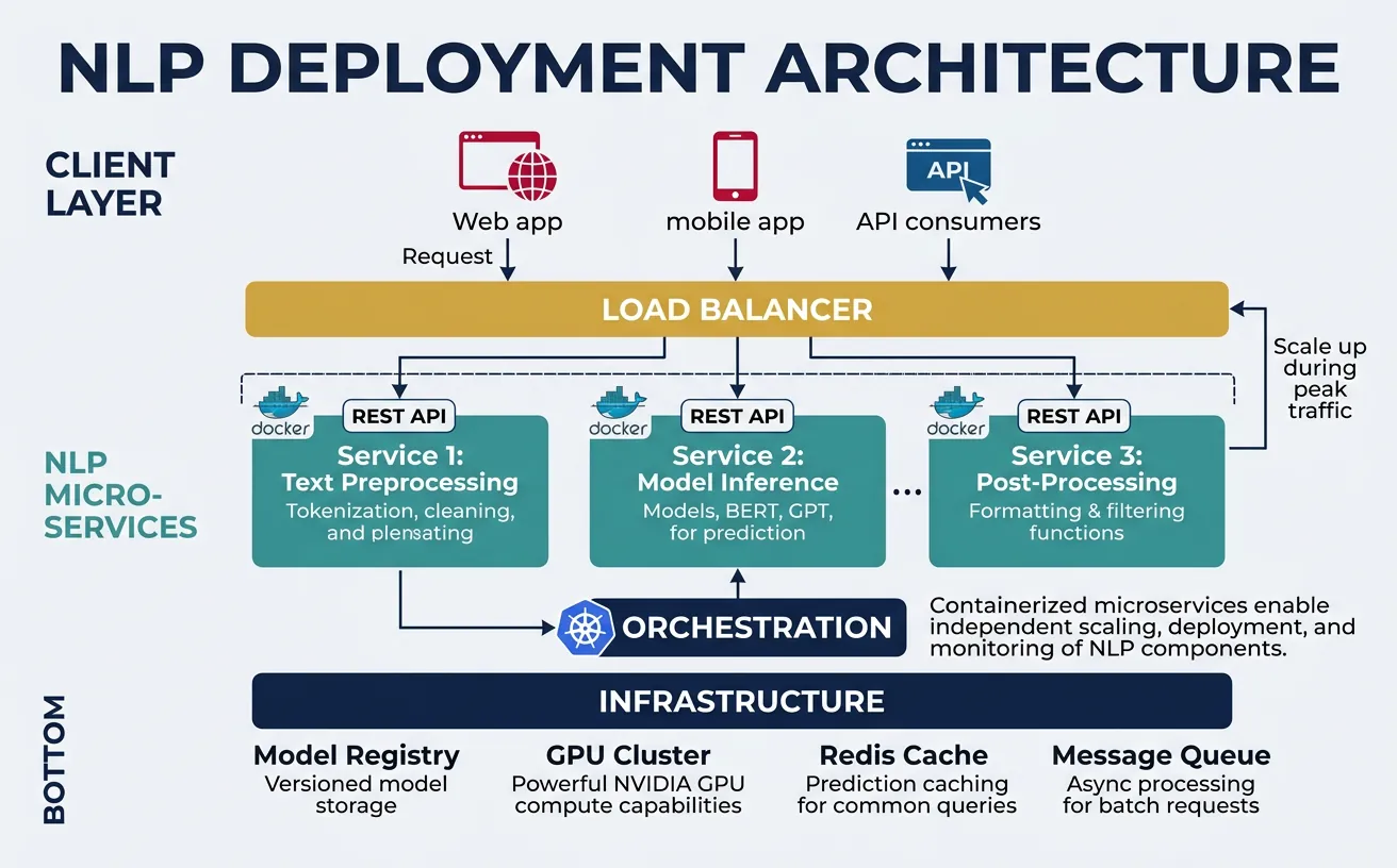
Deploying NLP models requires balancing performance, scalability, and operational complexity. The deployment strategy depends on latency requirements (real-time vs batch), scale (requests per second), cost constraints, and team expertise. Modern deployments typically use containerized microservices with GPU support, automated scaling, and comprehensive monitoring—but simpler approaches like serverless functions or managed ML platforms can be appropriate for smaller-scale applications.
Model Serving with FastAPI and ONNX
Model serving frameworks provide HTTP/gRPC endpoints for inference, handling request batching, model versioning, and hardware optimization. FastAPI offers a lightweight, high-performance solution for Python-based serving, while specialized frameworks like TorchServe, TensorFlow Serving, and Triton Inference Server provide advanced features like dynamic batching, model ensembling, and multi-model serving. ONNX Runtime is particularly effective for cross-platform deployment with consistent performance.
Key serving considerations include batching (grouping multiple requests for efficient GPU utilization), caching (avoiding redundant computation for repeated inputs), and model warmup (pre-loading models to eliminate cold-start latency). For transformer models, sequence padding strategies significantly impact throughput—sorting requests by length and using dynamic padding can improve batch efficiency by 2-3x.
# FastAPI NLP Model Server
from fastapi import FastAPI, HTTPException
from pydantic import BaseModel
from typing import List, Optional
import onnxruntime as ort
import numpy as np
from transformers import AutoTokenizer
import time

app = FastAPI(title="NLP Inference API", version="1.0.0")

# Global model and tokenizer (loaded once at startup)
class ModelServer:
    def __init__(self):
        self.tokenizer = None
        self.session = None
        self.model_loaded = False

    def load_model(self, model_path: str, tokenizer_name: str):
        """Load ONNX model and tokenizer"""
        self.tokenizer = AutoTokenizer.from_pretrained(tokenizer_name)
        self.session = ort.InferenceSession(
            model_path,
            providers=['CUDAExecutionProvider', 'CPUExecutionProvider']
        )
        self.model_loaded = True
        print(f"Model loaded from {model_path}")

    def predict(self, texts: List[str], max_length: int = 128):
        """Run inference on a batch of texts"""
        if not self.model_loaded:
            raise RuntimeError("Model not loaded")

        # Tokenize inputs
        inputs = self.tokenizer(
            texts,
            return_tensors="np",
            padding=True,
            truncation=True,
            max_length=max_length
        )

        # Run inference
        outputs = self.session.run(
            None,
            {
                "input_ids": inputs["input_ids"],
                "attention_mask": inputs["attention_mask"]
            }
        )

        return outputs[0]  # Return logits

server = ModelServer()

# Request/Response models
class PredictionRequest(BaseModel):
    texts: List[str]
    max_length: Optional[int] = 128

class PredictionResponse(BaseModel):
    predictions: List[int]
    probabilities: List[List[float]]
    latency_ms: float

@app.on_event("startup")
async def startup_event():
    # Load model at startup
    # server.load_model("model_quantized.onnx", "distilbert-base-uncased")
    print("Server started - load model with /load endpoint")

@app.post("/predict", response_model=PredictionResponse)
async def predict(request: PredictionRequest):
    """Run sentiment analysis on input texts"""
    start_time = time.time()

    try:
        logits = server.predict(request.texts, request.max_length)
        probabilities = np.exp(logits) / np.exp(logits).sum(axis=-1, keepdims=True)
        predictions = np.argmax(logits, axis=-1).tolist()

        latency = (time.time() - start_time) * 1000

        return PredictionResponse(
            predictions=predictions,
            probabilities=probabilities.tolist(),
            latency_ms=round(latency, 2)
        )
    except Exception as e:
        raise HTTPException(status_code=500, detail=str(e))

@app.get("/health")
async def health_check():
    return {"status": "healthy", "model_loaded": server.model_loaded}

# Run with: uvicorn server:app --host 0.0.0.0 --port 8000
print("FastAPI server code ready")
print("Endpoints: POST /predict, GET /health")
Serving Best Practices
Enable dynamic batching (batch_size=16-64, timeout=50ms), use async request handling, implement request queuing for load management, and always include health check endpoints for orchestration systems.
Containerization with Docker
Docker containers package models with all dependencies, ensuring consistent behavior across development, testing, and production environments. A well-designed container image includes the model artifacts, inference code, required libraries, and appropriate base image (use NVIDIA CUDA images for GPU inference). Multi-stage builds keep images small by separating build-time dependencies from runtime requirements.
Container best practices for NLP include: using specific version tags (not latest), minimizing image layers, implementing proper signal handling for graceful shutdown, and storing models externally (S3, GCS) rather than baking them into images. For large models, consider model caching volumes to avoid downloading on every container start.
# Dockerfile for NLP Model Serving (save as Dockerfile)
dockerfile_content = '''
# Multi-stage build for minimal image size
FROM python:3.10-slim as builder

WORKDIR /app

# Install build dependencies
RUN apt-get update && apt-get install -y --no-install-recommends \\
    build-essential \\
    && rm -rf /var/lib/apt/lists/*

# Install Python dependencies
COPY requirements.txt .
RUN pip install --no-cache-dir --user -r requirements.txt

# Production image
FROM python:3.10-slim

WORKDIR /app

# Copy installed packages from builder
COPY --from=builder /root/.local /root/.local
ENV PATH=/root/.local/bin:$PATH

# Copy application code
COPY app/ ./app/
COPY models/ ./models/

# Create non-root user for security
RUN useradd --create-home appuser
USER appuser

# Health check
HEALTHCHECK --interval=30s --timeout=10s --start-period=60s --retries=3 \\
    CMD curl -f http://localhost:8000/health || exit 1

# Run the server
EXPOSE 8000
CMD ["uvicorn", "app.server:app", "--host", "0.0.0.0", "--port", "8000"]
'''

requirements_content = '''
fastapi==0.104.1
uvicorn[standard]==0.24.0
onnxruntime==1.16.3
transformers==4.35.2
numpy==1.24.3
pydantic==2.5.2
'''

print("Dockerfile content:")
print(dockerfile_content[:500] + "...")
print("\nrequirements.txt content:")
print(requirements_content)
# Docker build and run commands (shell script)
docker_commands = """
# Build the image
docker build -t nlp-server:v1.0 .

# Run locally for testing
docker run -d \\
    --name nlp-server \\
    -p 8000:8000 \\
    -v $(pwd)/models:/app/models \\
    -e MODEL_PATH=/app/models/model.onnx \\
    -e TOKENIZER_NAME=distilbert-base-uncased \\
    nlp-server:v1.0

# Check logs
docker logs -f nlp-server

# Test the endpoint
curl -X POST http://localhost:8000/predict \\
    -H "Content-Type: application/json" \\
    -d '{"texts": ["This is great!", "This is terrible."]}'

# GPU support (requires nvidia-docker)
docker run -d \\
    --gpus all \\
    --name nlp-server-gpu \\
    -p 8000:8000 \\
    nlp-server:v1.0

# Push to registry
docker tag nlp-server:v1.0 myregistry.azurecr.io/nlp-server:v1.0
docker push myregistry.azurecr.io/nlp-server:v1.0
"""

print("Docker commands for NLP deployment:")
print(docker_commands)
Scaling & Load Balancing
Horizontal scaling adds more inference workers to handle increased load, while vertical scaling uses more powerful hardware (larger GPUs, more memory). Kubernetes orchestrates containerized deployments with automatic scaling based on CPU/GPU utilization, request queue depth, or custom metrics. For NLP workloads, GPU-aware scheduling ensures pods land on nodes with appropriate hardware, and resource limits prevent memory-hungry models from affecting co-located services.
Load balancing distributes requests across workers efficiently. For NLP, consider least-connections routing (prefer idle workers) over round-robin, as inference times vary significantly with input length. Implement request timeouts and circuit breakers to handle model failures gracefully. Auto-scaling should account for model warm-up time—scale up proactively based on traffic patterns rather than reactively when latency spikes.
# Kubernetes deployment configuration (save as deployment.yaml)
k8s_deployment = """
apiVersion: apps/v1
kind: Deployment
metadata:
  name: nlp-inference
  labels:
    app: nlp-inference
spec:
  replicas: 3
  selector:
    matchLabels:
      app: nlp-inference
  template:
    metadata:
      labels:
        app: nlp-inference
    spec:
      containers:
      - name: nlp-server
        image: myregistry.azurecr.io/nlp-server:v1.0
        ports:
        - containerPort: 8000
        resources:
          requests:
            memory: "2Gi"
            cpu: "1"
            nvidia.com/gpu: "1"
          limits:
            memory: "4Gi"
            cpu: "2"
            nvidia.com/gpu: "1"
        env:
        - name: MODEL_PATH
          value: "/models/model.onnx"
        - name: WORKERS
          value: "4"
        livenessProbe:
          httpGet:
            path: /health
            port: 8000
          initialDelaySeconds: 60
          periodSeconds: 10
        readinessProbe:
          httpGet:
            path: /health
            port: 8000
          initialDelaySeconds: 30
          periodSeconds: 5
        volumeMounts:
        - name: model-volume
          mountPath: /models
      volumes:
      - name: model-volume
        persistentVolumeClaim:
          claimName: model-pvc
---
apiVersion: v1
kind: Service
metadata:
  name: nlp-inference-service
spec:
  selector:
    app: nlp-inference
  ports:
  - port: 80
    targetPort: 8000
  type: LoadBalancer
"""

print("Kubernetes deployment configuration:")
print(k8s_deployment[:1500] + "...")
Horizontal Pod Autoscaler
Configure Kubernetes HPA to scale based on CPU utilization or custom metrics like request queue length for optimal resource usage.
# Horizontal Pod Autoscaler (save as hpa.yaml)
hpa_config = """
apiVersion: autoscaling/v2
kind: HorizontalPodAutoscaler
metadata:
  name: nlp-inference-hpa
spec:
  scaleTargetRef:
    apiVersion: apps/v1
    kind: Deployment
    name: nlp-inference
  minReplicas: 2
  maxReplicas: 10
  metrics:
  - type: Resource
    resource:
      name: cpu
      target:
        type: Utilization
        averageUtilization: 70
  - type: Pods
    pods:
      metric:
        name: inference_queue_depth
      target:
        type: AverageValue
        averageValue: "10"
  behavior:
    scaleUp:
      stabilizationWindowSeconds: 60
      policies:
      - type: Pods
        value: 2
        periodSeconds: 60
    scaleDown:
      stabilizationWindowSeconds: 300
      policies:
      - type: Percent
        value: 10
        periodSeconds: 60
"""
print("HPA configuration for NLP workloads:")
print(hpa_config)
MLOps for NLP
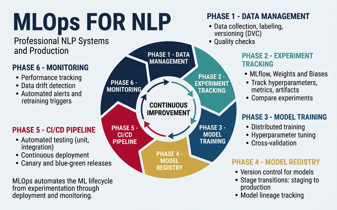
MLOps (Machine Learning Operations) brings DevOps practices to ML systems, automating the lifecycle from data preparation through model training, deployment, and monitoring. For NLP, MLOps addresses unique challenges: large model artifacts, expensive training runs, dataset versioning, and the need to track not just code but also data, hyperparameters, and model weights. A mature MLOps pipeline enables reproducible experiments, automated retraining, and confident production deployments.
Key MLOps components include: experiment tracking (logging metrics, parameters, and artifacts), model registry (versioned model storage with metadata), CI/CD pipelines (automated testing and deployment), and feature stores (centralized feature management). Tools like MLflow, Weights & Biases, and DVC integrate with NLP workflows, while cloud platforms (SageMaker, Vertex AI, Azure ML) provide managed MLOps infrastructure.
MLOps Maturity Levels
Level 0: Manual ML (notebooks) → Level 1: ML Pipeline Automation (automated training) → Level 2: CI/CD Pipeline Automation (automated testing/deployment) → Level 3: Full MLOps (automated retraining, monitoring, and drift detection). Most production NLP systems should target Level 2-3.
# MLflow experiment tracking for NLP
import mlflow
import mlflow.pytorch
from transformers import (
    AutoModelForSequenceClassification,
    AutoTokenizer,
    Trainer,
    TrainingArguments
)
import numpy as np
from sklearn.metrics import accuracy_score, f1_score

# Set up MLflow experiment
mlflow.set_tracking_uri("http://localhost:5000")  # MLflow server
mlflow.set_experiment("sentiment-classification")

def compute_metrics(eval_pred):
    """Compute metrics for evaluation"""
    predictions, labels = eval_pred
    predictions = np.argmax(predictions, axis=1)
    return {
        "accuracy": accuracy_score(labels, predictions),
        "f1": f1_score(labels, predictions, average="weighted")
    }

# Training function with MLflow tracking
def train_with_tracking(
    model_name: str,
    train_dataset,
    eval_dataset,
    num_epochs: int = 3,
    learning_rate: float = 2e-5,
    batch_size: int = 16
):
    with mlflow.start_run(run_name=f"train_{model_name}"):
        # Log parameters
        mlflow.log_params({
            "model_name": model_name,
            "num_epochs": num_epochs,
            "learning_rate": learning_rate,
            "batch_size": batch_size,
            "train_samples": len(train_dataset),
            "eval_samples": len(eval_dataset)
        })

        # Load model
        model = AutoModelForSequenceClassification.from_pretrained(
            model_name, num_labels=2
        )
        tokenizer = AutoTokenizer.from_pretrained(model_name)

        # Training arguments
        training_args = TrainingArguments(
            output_dir="./results",
            num_train_epochs=num_epochs,
            per_device_train_batch_size=batch_size,
            per_device_eval_batch_size=batch_size,
            learning_rate=learning_rate,
            evaluation_strategy="epoch",
            save_strategy="epoch",
            load_best_model_at_end=True,
            metric_for_best_model="f1"
        )

        # Train
        trainer = Trainer(
            model=model,
            args=training_args,
            train_dataset=train_dataset,
            eval_dataset=eval_dataset,
            compute_metrics=compute_metrics
        )

        trainer.train()

        # Log metrics
        eval_results = trainer.evaluate()
        mlflow.log_metrics(eval_results)

        # Log model artifact
        mlflow.pytorch.log_model(model, "model")
        mlflow.log_artifact("./results/training_args.bin")

        print(f"Run ID: {mlflow.active_run().info.run_id}")
        return model

print("MLflow training function ready")
print("Track experiments at http://localhost:5000")
# Model Registry with MLflow
import mlflow
from mlflow.tracking import MlflowClient

# Initialize MLflow client
client = MlflowClient()

def register_model(run_id: str, model_name: str, description: str = ""):
    """Register a trained model in the registry"""
    model_uri = f"runs:/{run_id}/model"

    # Register the model
    result = mlflow.register_model(
        model_uri=model_uri,
        name=model_name
    )

    # Add description
    client.update_registered_model(
        name=model_name,
        description=description
    )

    print(f"Model registered: {model_name} v{result.version}")
    return result

def promote_model(model_name: str, version: int, stage: str):
    """Promote model version to a stage (Staging, Production, Archived)"""
    client.transition_model_version_stage(
        name=model_name,
        version=version,
        stage=stage
    )
    print(f"Model {model_name} v{version} promoted to {stage}")

def load_production_model(model_name: str):
    """Load the production version of a model"""
    model_uri = f"models:/{model_name}/Production"
    model = mlflow.pytorch.load_model(model_uri)
    return model

# Example usage workflow
print("Model Registry Workflow:")
print("1. Train model → get run_id")
print("2. register_model(run_id, 'sentiment-classifier', 'BERT sentiment model')")
print("3. promote_model('sentiment-classifier', 1, 'Staging')")
print("4. Test in staging → promote_model('sentiment-classifier', 1, 'Production')")
print("5. load_production_model('sentiment-classifier') in serving code")
CI/CD Pipeline for NLP Models
Automate model testing and deployment with CI/CD pipelines. This GitHub Actions workflow tests model quality, builds containers, and deploys to Kubernetes.
# GitHub Actions workflow (.github/workflows/ml-pipeline.yml)
github_actions_yaml = """
name: NLP Model CI/CD

on:
  push:
    branches: [main]
    paths:
      - 'models/**'
      - 'src/**'
  pull_request:
    branches: [main]

jobs:
  test:
    runs-on: ubuntu-latest
    steps:
      - uses: actions/checkout@v3

      - name: Set up Python
        uses: actions/setup-python@v4
        with:
          python-version: '3.10'

      - name: Install dependencies
        run: pip install -r requirements.txt

      - name: Run unit tests
        run: pytest tests/ -v

      - name: Run model quality tests
        run: python tests/test_model_quality.py

  build:
    needs: test
    runs-on: ubuntu-latest
    if: github.ref == 'refs/heads/main'

    steps:
      - uses: actions/checkout@v3

      - name: Build Docker image
        run: |
          docker build -t nlp-server:${{ github.sha }} .
          docker tag nlp-server:${{ github.sha }} \\
            ${{ secrets.REGISTRY }}/nlp-server:${{ github.sha }}

      - name: Push to registry
        run: |
          echo ${{ secrets.REGISTRY_PASSWORD }} | docker login \\
            ${{ secrets.REGISTRY }} -u ${{ secrets.REGISTRY_USER }} --password-stdin
          docker push ${{ secrets.REGISTRY }}/nlp-server:${{ github.sha }}

  deploy:
    needs: build
    runs-on: ubuntu-latest

    steps:
      - name: Deploy to Kubernetes
        uses: azure/k8s-deploy@v4
        with:
          manifests: k8s/deployment.yaml
          images: ${{ secrets.REGISTRY }}/nlp-server:${{ github.sha }}
"""
print("GitHub Actions CI/CD pipeline:")
print(github_actions_yaml)
# DVC (Data Version Control) for dataset management
# Install: pip install dvc dvc-s3

# Initialize DVC in your project
# $ dvc init
# $ dvc remote add -d storage s3://my-bucket/dvc-cache

import subprocess
import json
from pathlib import Path

def setup_dvc_pipeline():
    """Create a DVC pipeline for NLP training"""

    # dvc.yaml defines the pipeline
    dvc_yaml = """
stages:
  preprocess:
    cmd: python src/preprocess.py
    deps:
      - data/raw/
      - src/preprocess.py
    outs:
      - data/processed/train.json
      - data/processed/test.json

  train:
    cmd: python src/train.py
    deps:
      - data/processed/train.json
      - src/train.py
      - configs/train_config.yaml
    params:
      - train_config.yaml:
          - model_name
          - learning_rate
          - num_epochs
    outs:
      - models/model.pt
    metrics:
      - metrics/train_metrics.json:
          cache: false

  evaluate:
    cmd: python src/evaluate.py
    deps:
      - data/processed/test.json
      - models/model.pt
      - src/evaluate.py
    metrics:
      - metrics/eval_metrics.json:
          cache: false
"""

    print("DVC Pipeline (dvc.yaml):")
    print(dvc_yaml)
    print("\nDVC Commands:")
    print("$ dvc repro          # Run/update pipeline")
    print("$ dvc push           # Push data/models to remote")
    print("$ dvc pull           # Pull data/models from remote")
    print("$ dvc metrics show   # Show metrics across experiments")
    print("$ dvc plots show     # Visualize metrics")

setup_dvc_pipeline()
Monitoring & Observability
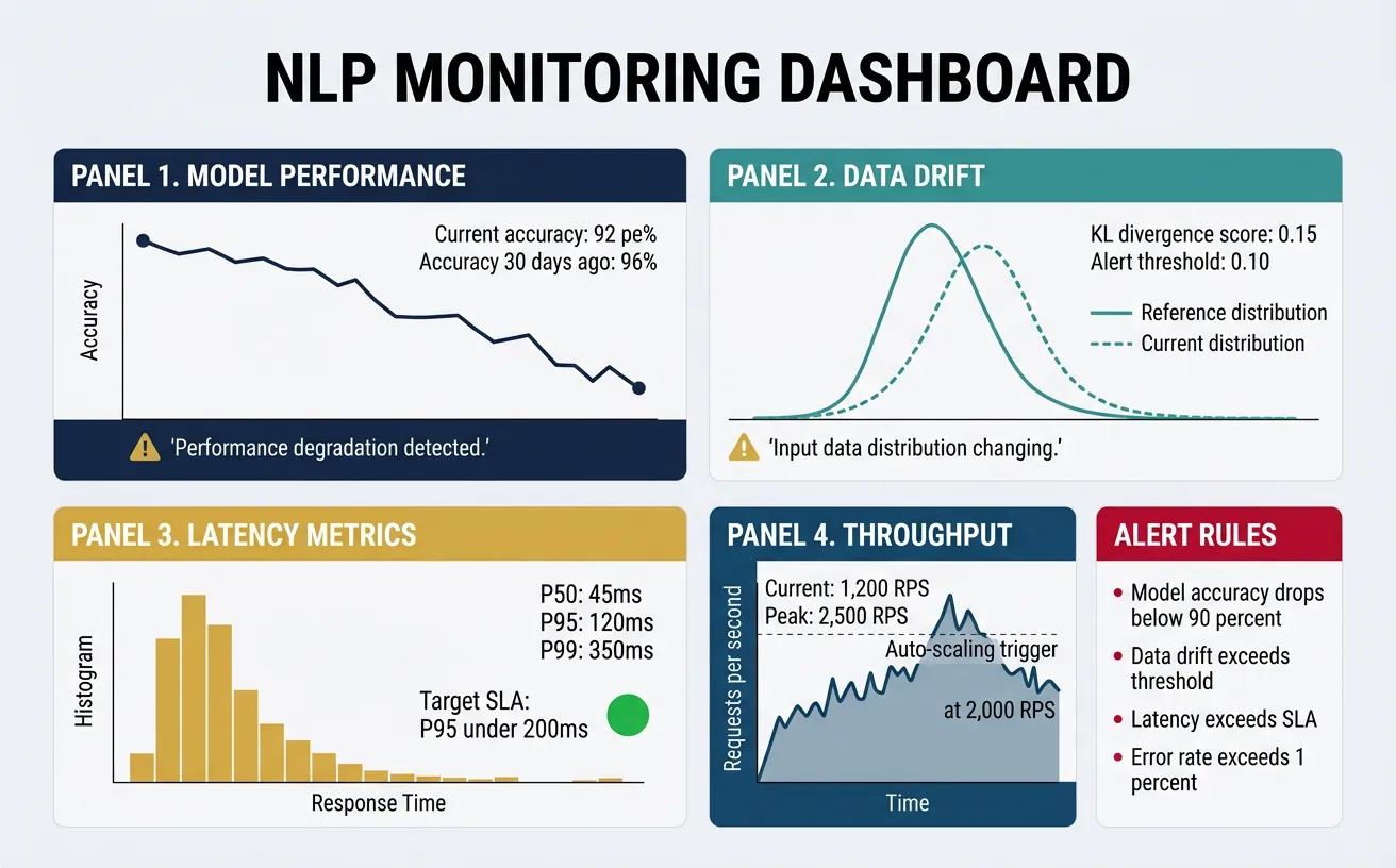
Production NLP systems require comprehensive monitoring to detect issues before they impact users. Beyond standard infrastructure metrics (CPU, memory, latency), NLP systems need model-specific monitoring: prediction distributions, confidence scores, input characteristics, and performance degradation over time. Observability encompasses metrics, logs, and traces—providing the visibility needed to understand system behavior and debug issues in complex ML pipelines.
Key monitoring areas include: data drift (input distribution changes), concept drift (relationship between inputs and outputs changes), model degradation (accuracy decline over time), and operational metrics (latency percentiles, error rates, throughput). Set up alerts for anomalies and establish baseline metrics during initial deployment. Regular model evaluation on fresh data helps detect drift before it significantly impacts performance.
Critical Alerts for NLP Systems
Set alerts for: p99 latency > threshold, error rate > 1%, prediction confidence distribution shift, input text length anomalies, and null/empty prediction rates. Review model performance weekly and retrain when accuracy drops below acceptable thresholds.
# Prometheus metrics for NLP model monitoring
from prometheus_client import Counter, Histogram, Gauge, start_http_server
import time
import numpy as np

# Define metrics
PREDICTION_COUNTER = Counter(
    'nlp_predictions_total',
    'Total number of predictions',
    ['model_name', 'prediction_class']
)

PREDICTION_LATENCY = Histogram(
    'nlp_prediction_latency_seconds',
    'Prediction latency in seconds',
    ['model_name'],
    buckets=[0.01, 0.025, 0.05, 0.1, 0.25, 0.5, 1.0, 2.5]
)

PREDICTION_CONFIDENCE = Histogram(
    'nlp_prediction_confidence',
    'Prediction confidence scores',
    ['model_name', 'prediction_class'],
    buckets=[0.5, 0.6, 0.7, 0.8, 0.9, 0.95, 0.99]
)

INPUT_LENGTH = Histogram(
    'nlp_input_length_tokens',
    'Input text length in tokens',
    ['model_name'],
    buckets=[10, 25, 50, 100, 200, 500]
)

MODEL_LOADED = Gauge(
    'nlp_model_loaded',
    'Whether the model is loaded (1) or not (0)',
    ['model_name', 'version']
)

class MetricsCollector:
    """Collect and expose model metrics"""

    def __init__(self, model_name: str, model_version: str):
        self.model_name = model_name
        self.model_version = model_version
        MODEL_LOADED.labels(model_name=model_name, version=model_version).set(1)

    def record_prediction(
        self,
        prediction_class: str,
        confidence: float,
        latency: float,
        input_length: int
    ):
        """Record metrics for a single prediction"""
        PREDICTION_COUNTER.labels(
            model_name=self.model_name,
            prediction_class=prediction_class
        ).inc()

        PREDICTION_LATENCY.labels(
            model_name=self.model_name
        ).observe(latency)

        PREDICTION_CONFIDENCE.labels(
            model_name=self.model_name,
            prediction_class=prediction_class
        ).observe(confidence)

        INPUT_LENGTH.labels(
            model_name=self.model_name
        ).observe(input_length)

# Example usage
collector = MetricsCollector("sentiment-bert", "v1.0")

# Simulate predictions
for _ in range(10):
    collector.record_prediction(
        prediction_class="positive",
        confidence=np.random.uniform(0.7, 0.99),
        latency=np.random.uniform(0.01, 0.1),
        input_length=np.random.randint(10, 200)
    )

print("Metrics collector initialized")
print("Start metrics server: start_http_server(8001)")
print("Scrape endpoint: http://localhost:8001/metrics")
# Data drift detection for NLP
import numpy as np
from scipy import stats
from collections import defaultdict
from typing import List, Dict
import hashlib

class DriftDetector:
    """Detect distribution shifts in NLP model inputs and outputs"""

    def __init__(self, window_size: int = 1000):
        self.window_size = window_size
        self.reference_stats = {}
        self.current_window = defaultdict(list)

    def compute_text_features(self, text: str) -> Dict[str, float]:
        """Extract statistical features from text"""
        words = text.split()
        return {
            "length": len(text),
            "word_count": len(words),
            "avg_word_length": np.mean([len(w) for w in words]) if words else 0,
            "unique_ratio": len(set(words)) / len(words) if words else 0,
        }

    def set_reference(self, texts: List[str]):
        """Set reference distribution from training/baseline data"""
        features = [self.compute_text_features(t) for t in texts]

        for key in features[0].keys():
            values = [f[key] for f in features]
            self.reference_stats[key] = {
                "mean": np.mean(values),
                "std": np.std(values),
                "values": values
            }

        print(f"Reference set with {len(texts)} samples")

    def add_sample(self, text: str) -> Dict[str, float]:
        """Add a sample and check for drift"""
        features = self.compute_text_features(text)

        for key, value in features.items():
            self.current_window[key].append(value)
            if len(self.current_window[key]) > self.window_size:
                self.current_window[key].pop(0)

        return features

    def detect_drift(self, significance: float = 0.05) -> Dict[str, Dict]:
        """Detect drift using statistical tests"""
        if not self.reference_stats:
            return {"error": "Reference not set"}

        results = {}
        for key in self.reference_stats.keys():
            if len(self.current_window[key]) < 100:
                results[key] = {"drift": False, "reason": "Insufficient samples"}
                continue

            # Kolmogorov-Smirnov test
            stat, p_value = stats.ks_2samp(
                self.reference_stats[key]["values"],
                self.current_window[key]
            )

            drift_detected = p_value < significance

            results[key] = {
                "drift": drift_detected,
                "p_value": p_value,
                "ks_statistic": stat,
                "reference_mean": self.reference_stats[key]["mean"],
                "current_mean": np.mean(self.current_window[key])
            }

        return results

# Example usage
detector = DriftDetector(window_size=500)

# Set reference from training data
reference_texts = [
    "This product is great",
    "Excellent service and quality",
    "Not satisfied with the purchase"
] * 100  # Simulate more data
detector.set_reference(reference_texts)

# Simulate production traffic (with drift)
production_texts = [
    "This is a much longer review with significantly more words than typical",
    "Another verbose customer review with extensive detail about the product"
] * 100

for text in production_texts[:200]:
    detector.add_sample(text)

# Check for drift
drift_results = detector.detect_drift()
for feature, result in drift_results.items():
    print(f"{feature}: drift={result.get('drift')}, p={result.get('p_value', 'N/A'):.4f}")
Grafana Dashboard for NLP Monitoring
Create comprehensive dashboards showing model health, performance trends, and drift indicators. Use Grafana with Prometheus for real-time monitoring.
# Grafana dashboard configuration (JSON)
grafana_dashboard = {
    "title": "NLP Model Monitoring",
    "panels": [
        {
            "title": "Prediction Latency (p50, p95, p99)",
            "type": "graph",
            "targets": [
                {"expr": "histogram_quantile(0.50, rate(nlp_prediction_latency_seconds_bucket[5m]))"},
                {"expr": "histogram_quantile(0.95, rate(nlp_prediction_latency_seconds_bucket[5m]))"},
                {"expr": "histogram_quantile(0.99, rate(nlp_prediction_latency_seconds_bucket[5m]))"}
            ]
        },
        {
            "title": "Predictions per Second",
            "type": "graph",
            "targets": [
                {"expr": "rate(nlp_predictions_total[1m])"}
            ]
        },
        {
            "title": "Prediction Distribution",
            "type": "piechart",
            "targets": [
                {"expr": "sum by (prediction_class) (nlp_predictions_total)"}
            ]
        },
        {
            "title": "Confidence Score Distribution",
            "type": "heatmap",
            "targets": [
                {"expr": "rate(nlp_prediction_confidence_bucket[5m])"}
            ]
        },
        {
            "title": "Input Length Trend",
            "type": "graph",
            "targets": [
                {"expr": "histogram_quantile(0.50, rate(nlp_input_length_tokens_bucket[5m]))"}
            ]
        }
    ],
    "alerts": [
        {
            "name": "High Latency Alert",
            "condition": "histogram_quantile(0.99, rate(nlp_prediction_latency_seconds_bucket[5m])) > 0.5",
            "severity": "critical"
        },
        {
            "name": "Low Confidence Alert",
            "condition": "avg(nlp_prediction_confidence) < 0.7",
            "severity": "warning"
        }
    ]
}

import json
print("Grafana Dashboard Configuration:")
print(json.dumps(grafana_dashboard, indent=2)[:1500] + "...")
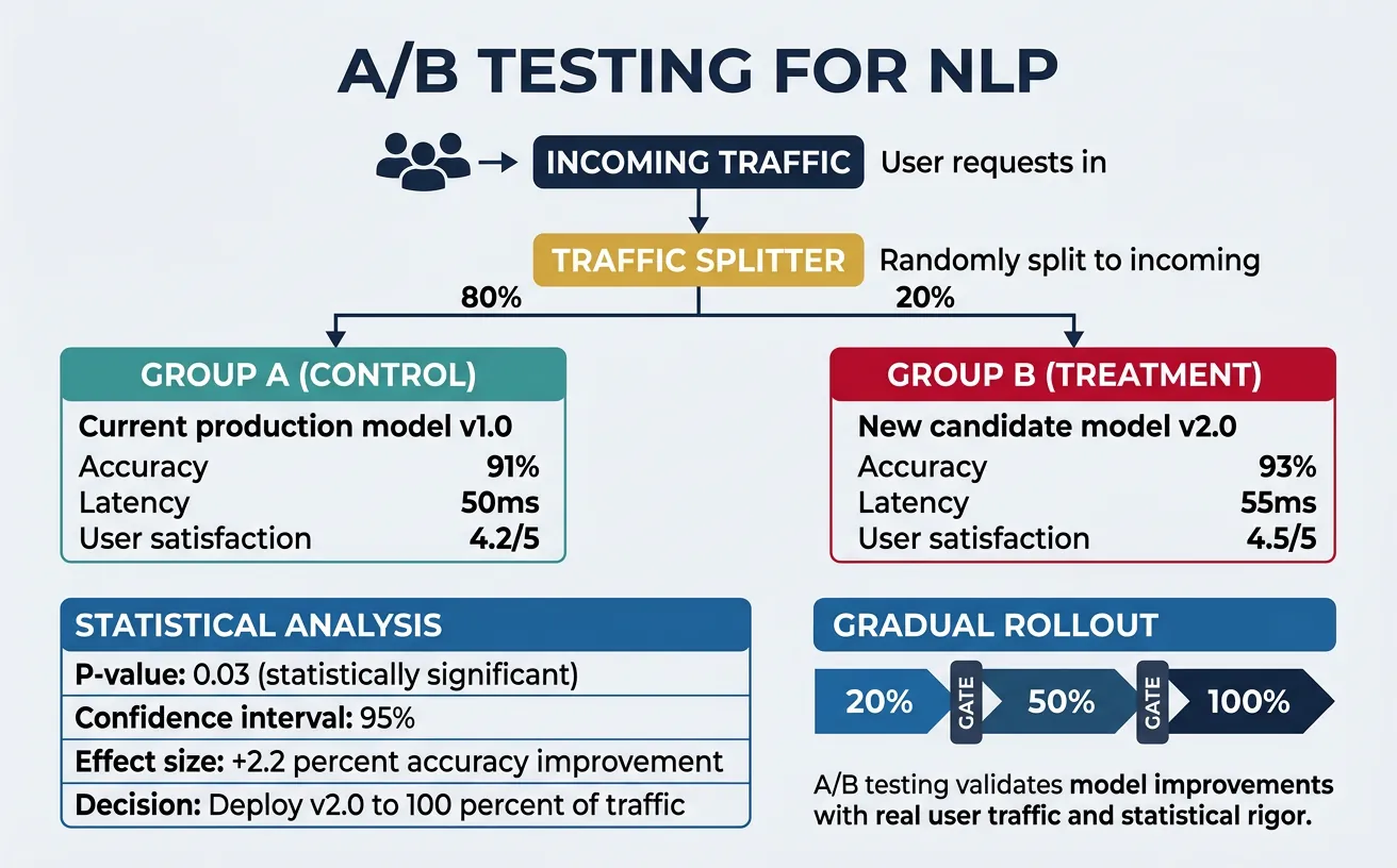
A/B Testing & Experimentation
A/B testing validates model improvements in production by comparing new models against the current baseline with real user traffic. Unlike offline evaluation, A/B tests measure actual business impact—user engagement, conversion rates, and satisfaction. For NLP systems, this is critical because offline metrics (accuracy, F1) don't always correlate with real-world performance. A chatbot might score high on benchmarks but frustrate users with its responses; A/B testing reveals such gaps.
Implement A/B testing with traffic splitting (route percentage of users to new model), metric collection (track both ML and business metrics), and statistical analysis (determine if differences are significant). Consider shadow mode deployment first—new model runs alongside production without serving users, allowing comparison without risk. Multi-armed bandit approaches can accelerate winner selection by dynamically allocating more traffic to better-performing variants.
A/B Testing Best Practices
Run tests for at least 2 weeks to capture weekly patterns, use at least 5% traffic per variant, define success metrics before starting, and ensure statistical significance (p < 0.05) before concluding. Don't peek at results and stop early—this inflates false positive rates.
# A/B Testing Framework for NLP Models
import random
import hashlib
from typing import Dict, Any, Optional
from dataclasses import dataclass
from datetime import datetime
import json

@dataclass
class Experiment:
    name: str
    variants: Dict[str, float]  # variant_name -> traffic_percentage
    start_time: datetime
    metrics: Dict[str, list]

class ABTestingFramework:
    """Framework for running A/B tests on NLP models"""

    def __init__(self):
        self.experiments: Dict[str, Experiment] = {}
        self.results: Dict[str, Dict] = {}

    def create_experiment(
        self,
        name: str,
        variants: Dict[str, float]
    ) -> Experiment:
        """Create a new A/B experiment"""
        # Validate traffic allocation
        total = sum(variants.values())
        if abs(total - 1.0) > 0.001:
            raise ValueError(f"Traffic must sum to 1.0, got {total}")

        experiment = Experiment(
            name=name,
            variants=variants,
            start_time=datetime.now(),
            metrics={v: [] for v in variants.keys()}
        )
        self.experiments[name] = experiment
        print(f"Created experiment '{name}' with variants: {variants}")
        return experiment

    def assign_variant(
        self,
        experiment_name: str,
        user_id: str
    ) -> str:
        """Consistently assign a user to a variant"""
        experiment = self.experiments.get(experiment_name)
        if not experiment:
            raise ValueError(f"Experiment '{experiment_name}' not found")

        # Hash user_id for consistent assignment
        hash_input = f"{experiment_name}:{user_id}"
        hash_value = int(hashlib.md5(hash_input.encode()).hexdigest(), 16)
        bucket = (hash_value % 10000) / 10000  # 0-1 range

        cumulative = 0
        for variant, percentage in experiment.variants.items():
            cumulative += percentage
            if bucket < cumulative:
                return variant

        return list(experiment.variants.keys())[-1]

    def record_metric(
        self,
        experiment_name: str,
        variant: str,
        metric_name: str,
        value: float
    ):
        """Record a metric observation for a variant"""
        experiment = self.experiments.get(experiment_name)
        if experiment:
            experiment.metrics[variant].append({
                "metric": metric_name,
                "value": value,
                "timestamp": datetime.now().isoformat()
            })

# Example: Model comparison A/B test
ab_framework = ABTestingFramework()

# Create experiment: 80% baseline, 20% new model
experiment = ab_framework.create_experiment(
    name="sentiment_model_v2",
    variants={
        "control": 0.80,   # Current production model
        "treatment": 0.20  # New optimized model
    }
)

# Simulate user assignment
users = [f"user_{i}" for i in range(100)]
assignments = {}
for user in users:
    variant = ab_framework.assign_variant("sentiment_model_v2", user)
    assignments[user] = variant

# Count assignments
from collections import Counter
print("\nAssignment distribution:")
print(Counter(assignments.values()))
# Statistical analysis for A/B test results
import numpy as np
from scipy import stats
from typing import List, Tuple

class ABTestAnalyzer:
    """Analyze A/B test results with statistical rigor"""

    @staticmethod
    def calculate_sample_size(
        baseline_rate: float,
        minimum_effect: float,
        alpha: float = 0.05,
        power: float = 0.8
    ) -> int:
        """Calculate required sample size for detecting an effect"""
        # Using formula for proportions
        p1 = baseline_rate
        p2 = baseline_rate * (1 + minimum_effect)
        p_avg = (p1 + p2) / 2

        z_alpha = stats.norm.ppf(1 - alpha / 2)
        z_beta = stats.norm.ppf(power)

        n = (2 * p_avg * (1 - p_avg) * (z_alpha + z_beta) ** 2) / (p2 - p1) ** 2
        return int(np.ceil(n))

    @staticmethod
    def compare_proportions(
        successes_a: int,
        total_a: int,
        successes_b: int,
        total_b: int
    ) -> Tuple[float, float, bool]:
        """Compare two proportions (e.g., conversion rates)"""
        p_a = successes_a / total_a
        p_b = successes_b / total_b

        # Pooled proportion
        p_pool = (successes_a + successes_b) / (total_a + total_b)

        # Standard error
        se = np.sqrt(p_pool * (1 - p_pool) * (1/total_a + 1/total_b))

        # Z-statistic
        z = (p_b - p_a) / se

        # Two-tailed p-value
        p_value = 2 * (1 - stats.norm.cdf(abs(z)))

        # Is it significant?
        significant = p_value < 0.05

        return p_a, p_b, p_value, significant

    @staticmethod
    def compare_means(
        values_a: List[float],
        values_b: List[float]
    ) -> Tuple[float, float, float, bool]:
        """Compare means using t-test (e.g., latency, satisfaction)"""
        mean_a = np.mean(values_a)
        mean_b = np.mean(values_b)

        # Welch's t-test (unequal variances)
        t_stat, p_value = stats.ttest_ind(values_a, values_b, equal_var=False)

        significant = p_value < 0.05

        return mean_a, mean_b, p_value, significant

# Example analysis
analyzer = ABTestAnalyzer()

# Calculate required sample size
# Baseline: 70% satisfaction, detect 5% relative improvement
sample_size = analyzer.calculate_sample_size(
    baseline_rate=0.70,
    minimum_effect=0.05,
    alpha=0.05,
    power=0.8
)
print(f"Required sample size per variant: {sample_size:,}")

# Simulate experiment results
np.random.seed(42)
control_satisfactions = np.random.binomial(1, 0.70, 5000)
treatment_satisfactions = np.random.binomial(1, 0.73, 5000)

# Analyze
p_a, p_b, p_value, significant = analyzer.compare_proportions(
    sum(control_satisfactions), len(control_satisfactions),
    sum(treatment_satisfactions), len(treatment_satisfactions)
)

print(f"\nSatisfaction Rate Analysis:")
print(f"Control: {p_a:.2%}")
print(f"Treatment: {p_b:.2%}")
print(f"Lift: {(p_b - p_a) / p_a:.2%}")
print(f"P-value: {p_value:.4f}")
print(f"Significant: {significant}")
Shadow Mode Deployment
Shadow mode runs the new model on production traffic without serving results. Compare predictions offline to validate before A/B testing.
# Shadow mode deployment
import asyncio
from typing import Dict, Any
import time

class ShadowModeDeployment:
    """Run shadow model alongside production for comparison"""

    def __init__(self, production_model, shadow_model):
        self.production = production_model
        self.shadow = shadow_model
        self.comparisons = []

    async def predict(self, input_data: Dict[str, Any]) -> Dict[str, Any]:
        """Make prediction and run shadow comparison"""
        start = time.time()

        # Production prediction (what user sees)
        prod_result = self.production.predict(input_data)
        prod_latency = time.time() - start

        # Shadow prediction (async, not blocking)
        shadow_start = time.time()
        shadow_result = self.shadow.predict(input_data)
        shadow_latency = time.time() - shadow_start

        # Log comparison (async to not affect response)
        comparison = {
            "input_hash": hash(str(input_data)),
            "production_prediction": prod_result,
            "shadow_prediction": shadow_result,
            "agreement": prod_result == shadow_result,
            "prod_latency": prod_latency,
            "shadow_latency": shadow_latency
        }
        self.comparisons.append(comparison)

        # Return only production result
        return prod_result

    def get_comparison_stats(self) -> Dict[str, float]:
        """Get shadow comparison statistics"""
        if not self.comparisons:
            return {}

        agreements = [c["agreement"] for c in self.comparisons]
        prod_latencies = [c["prod_latency"] for c in self.comparisons]
        shadow_latencies = [c["shadow_latency"] for c in self.comparisons]

        return {
            "total_comparisons": len(self.comparisons),
            "agreement_rate": sum(agreements) / len(agreements),
            "avg_prod_latency": sum(prod_latencies) / len(prod_latencies),
            "avg_shadow_latency": sum(shadow_latencies) / len(shadow_latencies)
        }

print("Shadow mode deployment ready")
print("Usage: shadow = ShadowModeDeployment(prod_model, new_model)")
print("       result = await shadow.predict(input)")
print("       stats = shadow.get_comparison_stats()")
Conclusion & Next Steps
Deploying NLP models to production is as much an engineering challenge as a machine learning one. We've covered the complete lifecycle: optimization techniques (quantization, distillation, pruning) to reduce model size and latency; deployment strategies (containerization, serving frameworks, Kubernetes scaling); MLOps practices (experiment tracking, model registry, CI/CD); and monitoring (metrics, drift detection, alerting). These components work together to create reliable, maintainable NLP systems that serve real users at scale.
The key takeaways are: (1) Start simple—deploy with FastAPI/ONNX before investing in complex infrastructure; (2) Optimize incrementally—measure baseline latency, then apply quantization/distillation as needed; (3) Monitor everything—ML systems fail silently without proper observability; (4) Automate aggressively—manual deployments don't scale; (5) Validate in production—A/B testing is the ground truth for model improvements.
Production NLP Checklist
Before going live: ✅ Model optimized (latency < threshold) ✅ Container tested locally ✅ Health checks implemented ✅ Metrics/logging configured ✅ Alerts set up ✅ Rollback plan documented ✅ Shadow mode validation passed ✅ Load testing completed ✅ Model versioned in registry
Your Production NLP Journey
- Week 1-2: Optimize your model with dynamic quantization. Measure latency/accuracy trade-offs. Export to ONNX format.
- Week 3-4: Build FastAPI serving endpoint. Containerize with Docker. Test locally with realistic traffic patterns.
- Week 5-6: Set up Prometheus metrics and Grafana dashboards. Implement drift detection for your specific data distribution.
- Week 7-8: Deploy to Kubernetes (or managed ML platform). Configure auto-scaling. Run shadow mode comparison.
- Week 9-10: Launch A/B test with 10% traffic. Define success metrics. Analyze results with statistical rigor.
- Ongoing: Monitor drift weekly. Retrain monthly or when performance drops. Iterate on optimization as traffic grows.
This completes Part 15 of our NLP series. You now have the knowledge to take models from notebooks to production with confidence. In the final part, we'll explore cutting-edge research and future directions in NLP—multimodal models, efficient transformers, and the frontiers of language AI.