Robotics & Automation Series Part 15: Advanced & Emerging Robotics

Soft Robotics

Think of traditional robots as skeletons — rigid, strong, and precise. Now imagine a robot built more like an octopus tentacle: it can squeeze through cracks, gently wrap around a tomato, and conform to irregular surfaces. That is the promise of soft robotics, a field that replaces metal links with elastomers, silicones, and fabric-based structures.

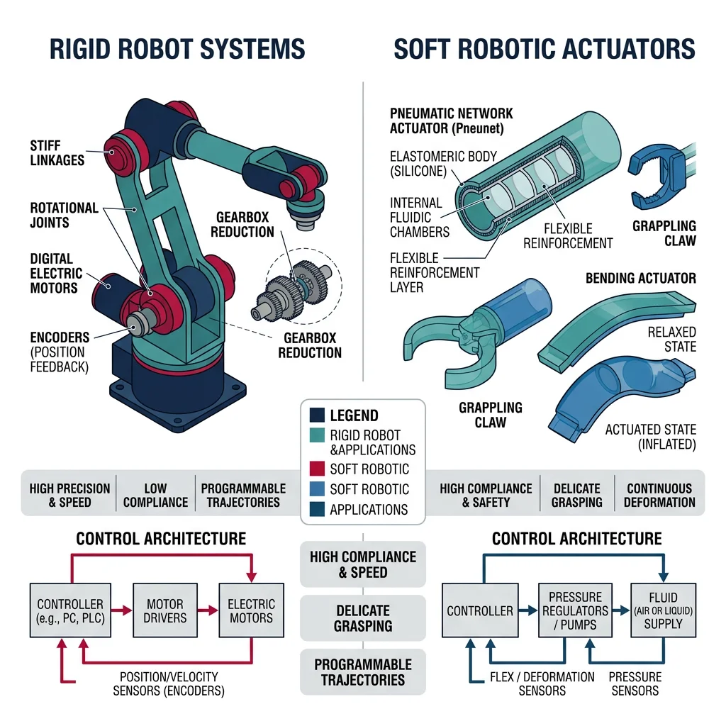
Compliant Materials

Soft robots are built from materials with elastic moduli closer to biological tissue (kPa–MPa range) rather than metals (GPa range). Key material families include:

Material Class	Examples	Young's Modulus	Typical Use
Silicone Elastomers	Ecoflex, Dragon Skin	10–100 kPa	Pneumatic actuators, grippers
Shape Memory Alloys	Nitinol (NiTi)	28–83 GPa (variable)	Bending actuators, stents
Hydrogels	PAAm, PNIPAM	1–100 kPa	Drug delivery, micro-robots
Electroactive Polymers	PVDF, acrylic DE	0.1–10 MPa	Artificial muscles
Fabric/Textile	Nylon, Kevlar composites	1–10 GPa	Wearable exosuits

Continuum Kinematics

Unlike rigid robots with discrete joints, soft robots deform continuously. The Piecewise Constant Curvature (PCC) model approximates a soft body as a series of circular arcs, each described by curvature κ, arc length s, and bending plane angle φ:

import numpy as np
import matplotlib.pyplot as plt

def pcc_arc(kappa, s, phi, n_points=50):
    """Compute 3D arc using Piecewise Constant Curvature model.
    kappa: curvature (1/m), s: arc length (m), phi: bending plane angle (rad)
    """
    if abs(kappa) < 1e-9:
        # Straight segment
        t = np.linspace(0, s, n_points)
        return np.zeros(n_points), np.zeros(n_points), t

    theta = np.linspace(0, kappa * s, n_points)
    r = 1.0 / kappa
    x = r * (1 - np.cos(theta)) * np.cos(phi)
    y = r * (1 - np.cos(theta)) * np.sin(phi)
    z = r * np.sin(theta)
    return x, y, z

# Two-segment soft robot arm
fig = plt.figure(figsize=(8, 6))
ax = fig.add_subplot(111, projection='3d')

# Segment 1: gentle bend
x1, y1, z1 = pcc_arc(kappa=3.0, s=0.15, phi=0)
ax.plot(x1, y1, z1, 'b-', linewidth=4, label='Segment 1 (κ=3)')

# Segment 2: tighter bend from endpoint of seg 1
x2, y2, z2 = pcc_arc(kappa=6.0, s=0.10, phi=np.pi/4)
ax.plot(x2 + x1[-1], y2 + y1[-1], z2 + z1[-1], 'r-', linewidth=4, label='Segment 2 (κ=6)')

ax.set_xlabel('X (m)')
ax.set_ylabel('Y (m)')
ax.set_zlabel('Z (m)')
ax.set_title('Piecewise Constant Curvature — 2-Segment Soft Robot')
ax.legend()
plt.tight_layout()
plt.show()

Pneumatic Soft Actuators

The most popular actuation method in soft robotics is pneumatic actuation — inflating or deflating air chambers embedded in an elastomeric body. The geometry of internal voids determines the motion: asymmetric chambers produce bending, concentric chambers produce elongation, and helical chambers produce twisting.

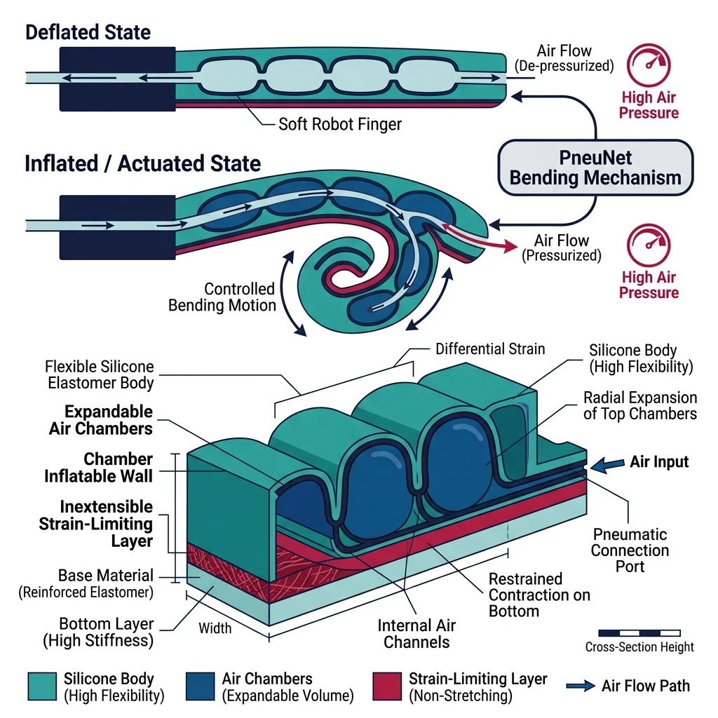
PneuNet (Pneumatic Network) Actuators

A PneuNet actuator consists of a series of connected air chambers cast in silicone with an inextensible strain-limiting layer on one side. When pressurized, the extensible top expands while the bottom constrains, causing the actuator to curl — much like a bimetallic strip heated on one side.

import numpy as np
import matplotlib.pyplot as plt

def pneunet_bending(pressure_kpa, n_chambers=5, chamber_height=0.01,
                     wall_thickness=0.002, E_silicone=100e3):
    """Simplified PneuNet bending angle prediction.
    pressure_kpa: input pressure in kPa
    Returns: total bending angle in degrees
    """
    pressure_pa = pressure_kpa * 1000
    # Each chamber contributes an angular deflection
    # theta_i ≈ (P * h) / (E * t) for thin-walled approximation
    theta_per_chamber = (pressure_pa * chamber_height) / (E_silicone * wall_thickness)
    total_angle_rad = n_chambers * theta_per_chamber
    return np.degrees(total_angle_rad)

pressures = np.linspace(0, 80, 100)
angles = [pneunet_bending(p) for p in pressures]

plt.figure(figsize=(8, 5))
plt.plot(pressures, angles, 'b-', linewidth=2)
plt.xlabel('Input Pressure (kPa)')
plt.ylabel('Bending Angle (degrees)')
plt.title('PneuNet Actuator: Pressure vs. Bending Response')
plt.grid(True, alpha=0.3)
plt.axhline(y=180, color='r', linestyle='--', alpha=0.5, label='180° max curl')
plt.legend()
plt.tight_layout()
plt.show()
print(f"Angle at 40 kPa: {pneunet_bending(40):.1f}°")
print(f"Angle at 70 kPa: {pneunet_bending(70):.1f}°")

Soft Grippers & Manipulation

Soft grippers exploit compliance to conform around objects of unknown shape, distributing contact forces naturally. This makes them ideal for picking fruit, handling electronics, and food processing — tasks where rigid grippers require expensive force sensors and complex control.

Gripper Architectures

Type	Mechanism	Payload	Best For
Fin Ray	Passive compliance — fingers bend inward on contact	0.1–5 kg	Delicate objects, irregular shapes
Granular Jamming	Bag of granules vacuum-sealed around object	1–20 kg	Universal grasping, unknown objects
PneuNet Fingers	Pneumatic chambers curl fingers around object	0.05–2 kg	Lab automation, food handling
Gecko-Inspired	Van der Waals adhesion via micro-structured surfaces	0.01–1 kg	Flat/smooth surfaces, space debris
Electroadhesion	Electrostatic attraction via charged electrodes	0.01–5 kg	Textiles, paper, thin materials

import numpy as np
import matplotlib.pyplot as plt

def granular_jamming_force(vacuum_kpa, bag_area_m2=0.01, friction_coeff=0.6):
    """Estimate holding force of a granular jamming gripper.
    F_hold ≈ μ × P × A (Coulomb friction model)
    vacuum_kpa: gauge vacuum pressure (kPa)
    """
    pressure_pa = vacuum_kpa * 1000
    return friction_coeff * pressure_pa * bag_area_m2

# Compare gripper types
vacuums = np.linspace(0, 80, 100)
forces = [granular_jamming_force(v) for v in vacuums]

plt.figure(figsize=(8, 5))
plt.plot(vacuums, forces, 'g-', linewidth=2, label='Granular Jamming')
plt.axhline(y=9.81 * 1, color='r', linestyle='--', alpha=0.6, label='1 kg object weight')
plt.axhline(y=9.81 * 5, color='orange', linestyle='--', alpha=0.6, label='5 kg object weight')
plt.xlabel('Vacuum Pressure (kPa)')
plt.ylabel('Holding Force (N)')
plt.title('Granular Jamming Gripper: Holding Force vs. Vacuum')
plt.legend()
plt.grid(True, alpha=0.3)
plt.tight_layout()
plt.show()
print(f"At 60 kPa vacuum: {granular_jamming_force(60):.1f} N holding force")

Bio-Inspired Robotics

Nature has had billions of years of R&D. Bio-inspired robotics (biomimetics) studies biological organisms and adapts their strategies — locomotion gaits, sensing modalities, material properties, and collective behaviors — into engineered systems. The goal isn't to copy nature exactly, but to extract design principles that evolution has optimized.

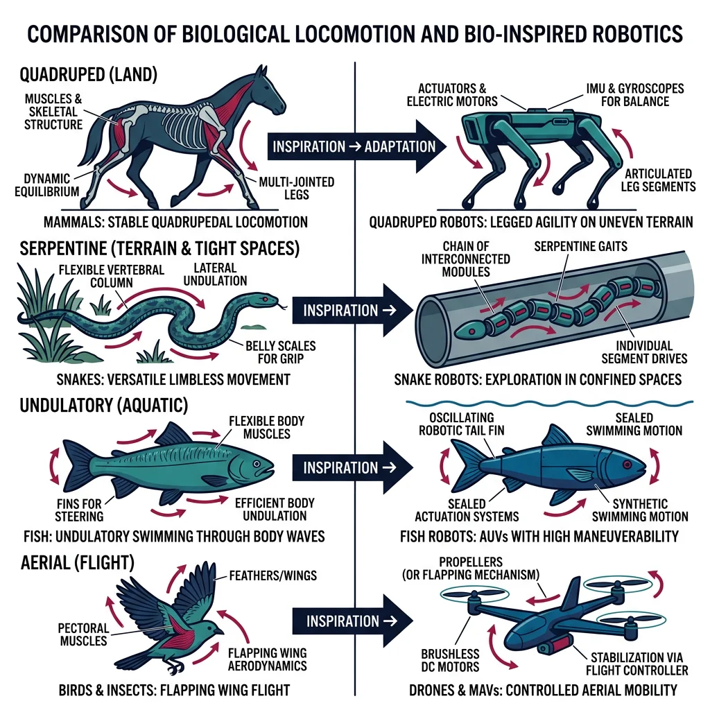
Locomotion Strategies from Nature

Organism	Locomotion	Robot Example	Key Advantage
Cheetah	Bounding gait, flexible spine	MIT Cheetah 3	High-speed terrain traversal
Gecko	Wall climbing via setae adhesion	Stickybot (Stanford)	Vertical surface mobility
Snake	Lateral undulation, sidewinding	CMU Snake Robot	Confined space navigation
Cockroach	Rapid alternating tripod gait	DASH, RHex	Obstacle traversal at small scale
Fish	Carangiform / thunniform swimming	MIT RoboTuna, SoFi	Efficient underwater propulsion
Bird	Flapping flight, soaring	Festo SmartBird	Agile aerial maneuvering

Artificial Muscles

Biological muscles are remarkable actuators — they are soft, lightweight, self-healing, and can generate forces up to 0.35 MPa specific stress. Engineering artificial muscles aims to match these properties for robots that move more naturally than servo-driven linkages.

Artificial Muscle Technologies

Technology	Mechanism	Strain (%)	Specific Stress (MPa)	Response Time
Dielectric Elastomer (DEA)	Electrostatic compression of elastomer film	10–100	0.1–3	ms
Shape Memory Alloy (SMA)	Phase transformation (martensite↔austenite)	4–8	200–700	0.1–10 s
Pneumatic Artificial Muscle (PAM)	Braided mesh contracts when pressurized	20–40	0.1–0.5	10–100 ms
Twisted Coiled Polymer (TCP)	Nylon fiber untwists when heated	20–50	5–30	0.5–5 s
Hydraulic Amplification (HASEL)	Electrostatic zipping displaces fluid	10–50	0.1–1	ms

import numpy as np
import matplotlib.pyplot as plt

def mckibben_force(pressure_kpa, braid_angle_deg=20, radius=0.01):
    """McKibben pneumatic artificial muscle force model.
    F = (P × π × r²) × (3 × cos²(θ) - 1) / (4π × n²)
    Simplified: F ≈ P × A × (3cos²θ - 1)
    """
    P = pressure_kpa * 1000  # Pa
    theta = np.radians(braid_angle_deg)
    A = np.pi * radius**2
    force = P * A * (3 * np.cos(theta)**2 - 1)
    return max(force, 0)

pressures = np.linspace(0, 600, 100)
angles = [15, 20, 25, 30]

plt.figure(figsize=(9, 5))
for angle in angles:
    forces = [mckibben_force(p, angle) for p in pressures]
    plt.plot(pressures, forces, linewidth=2, label=f'Braid angle {angle}°')

plt.xlabel('Pressure (kPa)')
plt.ylabel('Contraction Force (N)')
plt.title('McKibben Muscle: Force vs. Pressure at Different Braid Angles')
plt.legend()
plt.grid(True, alpha=0.3)
plt.tight_layout()
plt.show()
print(f"Force at 400 kPa, 20° braid: {mckibben_force(400, 20):.2f} N")

Swarm & Collective Behavior

A single ant cannot carry much, but a colony of ants builds bridges, farms fungus, and wages wars. Swarm robotics takes this principle — simple individuals, complex collective behavior — and applies it to groups of robots that communicate locally, share no central controller, and achieve emergent coordination.

import numpy as np
import matplotlib.pyplot as plt

def simulate_boids(n_boids=40, steps=200, separation_r=0.1,
                    alignment_r=0.3, cohesion_r=0.5):
    """Reynolds Boids flocking simulation.
    3 rules: separation, alignment, cohesion.
    """
    # Initialize positions and velocities
    pos = np.random.rand(n_boids, 2)
    vel = (np.random.rand(n_boids, 2) - 0.5) * 0.02
    history = [pos.copy()]

    for step in range(steps):
        new_vel = vel.copy()
        for i in range(n_boids):
            diffs = pos - pos[i]
            dists = np.linalg.norm(diffs, axis=1)
            dists[i] = np.inf  # exclude self

            # Rule 1: Separation — steer away from close neighbors
            sep_mask = dists < separation_r
            if sep_mask.any():
                new_vel[i] -= diffs[sep_mask].mean(axis=0) * 0.05

            # Rule 2: Alignment — match velocity of nearby boids
            align_mask = dists < alignment_r
            if align_mask.any():
                new_vel[i] += (vel[align_mask].mean(axis=0) - vel[i]) * 0.05

            # Rule 3: Cohesion — steer towards center of nearby group
            coh_mask = dists < cohesion_r
            if coh_mask.any():
                center = pos[coh_mask].mean(axis=0)
                new_vel[i] += (center - pos[i]) * 0.01

        # Limit speed
        speeds = np.linalg.norm(new_vel, axis=1, keepdims=True)
        max_speed = 0.02
        new_vel = np.where(speeds > max_speed, new_vel / speeds * max_speed, new_vel)

        vel = new_vel
        pos = pos + vel
        pos = pos % 1.0  # wrap around
        history.append(pos.copy())

    return history

history = simulate_boids(n_boids=40, steps=150)

fig, axes = plt.subplots(1, 3, figsize=(14, 4))
for idx, (step, title) in enumerate([(0, 'Initial (Random)'), (50, 'Forming Flocks'), (149, 'Stable Flocking')]):
    ax = axes[idx]
    ax.scatter(history[step][:, 0], history[step][:, 1], s=20, c='teal', alpha=0.8)
    ax.set_xlim(0, 1)
    ax.set_ylim(0, 1)
    ax.set_title(title)
    ax.set_aspect('equal')
    ax.grid(True, alpha=0.2)
plt.suptitle('Reynolds Boids: Emergent Flocking from 3 Simple Rules', fontsize=13)
plt.tight_layout()
plt.show()
print("Swarm behaviors: separation + alignment + cohesion = emergent flocking")

Medical & Surgical Robotics

Medical robotics is transforming healthcare — from surgeries performed with sub-millimeter precision through tiny incisions, to rehabilitation exoskeletons that help stroke patients walk again, to microscopic robots that could one day deliver drugs directly to cancer cells. This field demands the highest standards of safety, precision, and regulatory compliance.

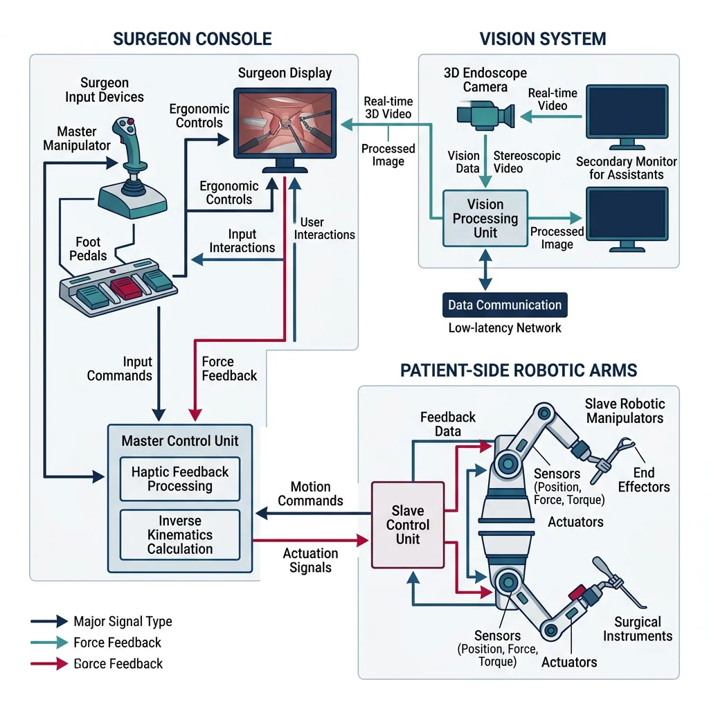
Surgical Robot Architectures

System	Manufacturer	Type	Specialties	Installations
da Vinci Xi	Intuitive Surgical	Teleoperated	Urology, gynecology, general	~7,500+
ROSA ONE	Zimmer Biomet	Semi-autonomous	Neurosurgery, spine	~800+
Mako SmartRobotics	Stryker	Haptic-guided	Orthopedic (joint replacement)	~2,000+
Ion Bronchoscopy	Intuitive Surgical	Shape-sensing catheter	Lung biopsy	~400+
Hugo RAS	Medtronic	Modular teleoperated	General, urological	~200+ (growing)

import numpy as np
import matplotlib.pyplot as plt

def tremor_filter(signal, cutoff_hz=6, dt=0.001):
    """Simple low-pass filter to simulate surgical tremor elimination.
    Removes frequencies above cutoff_hz (hand tremor is typically 8-12 Hz).
    Uses exponential moving average as simple approximation.
    """
    alpha = dt * cutoff_hz * 2 * np.pi / (1 + dt * cutoff_hz * 2 * np.pi)
    filtered = np.zeros_like(signal)
    filtered[0] = signal[0]
    for i in range(1, len(signal)):
        filtered[i] = alpha * signal[i] + (1 - alpha) * filtered[i-1]
    return filtered

# Simulate surgeon hand movement + tremor
t = np.linspace(0, 2, 2000)
dt = t[1] - t[0]
intended_motion = 0.01 * np.sin(2 * np.pi * 0.5 * t)  # Slow intended movement (0.5 Hz)
tremor = 0.0001 * np.sin(2 * np.pi * 10 * t + 0.3)     # 10 Hz hand tremor (100 μm)
hand_signal = intended_motion + tremor

# Apply motion scaling (5:1) and tremor filter
scaled_signal = hand_signal / 5.0  # 5:1 scaling
filtered_signal = tremor_filter(scaled_signal, cutoff_hz=6, dt=dt)

fig, axes = plt.subplots(3, 1, figsize=(10, 7), sharex=True)
axes[0].plot(t, hand_signal * 1000, 'r-', linewidth=1)
axes[0].set_ylabel('mm')
axes[0].set_title('Surgeon Hand Motion (with 10 Hz tremor)')

axes[1].plot(t, scaled_signal * 1000, 'orange', linewidth=1)
axes[1].set_ylabel('mm')
axes[1].set_title('After 5:1 Motion Scaling')

axes[2].plot(t, filtered_signal * 1000, 'g-', linewidth=1.5)
axes[2].set_ylabel('mm')
axes[2].set_title('After Tremor Filtration (6 Hz cutoff)')
axes[2].set_xlabel('Time (s)')

for ax in axes:
    ax.grid(True, alpha=0.3)
plt.suptitle('Surgical Robot: Motion Scaling + Tremor Filtration Pipeline', fontsize=13)
plt.tight_layout()
plt.show()
print(f"Tremor amplitude: {np.std(tremor)*1e6:.0f} μm → After filtering: {np.std(filtered_signal - tremor_filter(intended_motion/5, 6, dt))*1e6:.1f} μm")

Rehabilitation Robotics

After stroke, spinal cord injury, or limb amputation, rehabilitation robots help patients regain motor function through repetitive, precisely controlled exercises. Unlike a human therapist limited by fatigue and inconsistency, a robot can deliver thousands of identical training repetitions per session while measuring progress with sensor-level precision.

Rehabilitation Robot Categories

Category	Example	Application	Mechanism
Upper-limb Exoskeleton	Armeo Spring (Hocoma)	Stroke arm recovery	Gravity compensation + guided movement
Lower-limb Exoskeleton	ReWalk, Ekso GT	Spinal cord injury walking	Powered hip/knee joints + crutches
Gait Trainer	Lokomat (Hocoma)	Treadmill-based gait retraining	Body-weight support + leg guidance
End-Effector	MIT-Manus / InMotion ARM	Planar reaching exercises	Patient holds handle, robot guides/resists
Prosthetic Hand	LUKE Arm, bebionic	Amputee dexterity	Myoelectric signals drive motorized fingers

Micro & Nano Robots for Medicine

Imagine swallowing a robot the size of a grain of sand that navigates your bloodstream, finds a tumor, and delivers chemotherapy directly to cancer cells — sparing healthy tissue from toxic side effects. This is the vision of micro/nano robotics, a field operating at scales from 1 μm to 1 mm.

Propulsion Mechanisms at Micro-Scale

At microscopic scales, inertia is negligible and viscous forces dominate (low Reynolds number Re < 1). Swimming strategies that work for fish fail completely. Micro-robots use alternative propulsion:

Propulsion	Mechanism	Control	Speed
Magnetic Helical	Rotating helical body in external magnetic field	Rotating magnets	1–50 body lengths/s
Catalytic Janus	Asymmetric H₂O₂ decomposition creates bubble thrust	Chemical gradient	5–30 μm/s
Acoustic	Ultrasound-driven bubble oscillation	Frequency tuning	10–100 μm/s
Biohybrid	Sperm cells or bacteria attached to synthetic body	Magnetic + chemical	20–100 μm/s
Light-Driven	Photocatalytic reaction on one face	Laser steering	1–20 μm/s

import numpy as np
import matplotlib.pyplot as plt

def helical_microbot_velocity(freq_hz, helix_radius_um=5, pitch_um=20,
                                viscosity=0.001, body_length_um=50):
    """Estimate velocity of a magnetically actuated helical micro-swimmer.
    Uses resistive force theory (Cox, 1970) simplified model.
    v ≈ (2π × f × p × ξ_perp) / (ξ_para + ξ_perp)
    where p = pitch, ξ = drag coefficients
    """
    # Convert to SI
    p = pitch_um * 1e-6
    r_h = helix_radius_um * 1e-6
    L = body_length_um * 1e-6

    # Drag coefficients (slender body theory)
    ln_term = np.log(2 * L / (2 * r_h))
    xi_para = 2 * np.pi * viscosity / (ln_term - 0.5)
    xi_perp = 4 * np.pi * viscosity / (ln_term + 0.5)

    # Swimming velocity
    omega = 2 * np.pi * freq_hz
    v = (omega * p * (xi_perp - xi_para)) / (xi_para + xi_perp)
    return abs(v) * 1e6  # return in μm/s

frequencies = np.linspace(1, 100, 100)
pitches = [10, 20, 40]

plt.figure(figsize=(9, 5))
for p in pitches:
    velocities = [helical_microbot_velocity(f, pitch_um=p) for f in frequencies]
    plt.plot(frequencies, velocities, linewidth=2, label=f'Pitch = {p} μm')

plt.xlabel('Rotation Frequency (Hz)')
plt.ylabel('Swimming Speed (μm/s)')
plt.title('Helical Micro-Robot: Speed vs. Magnetic Field Rotation Frequency')
plt.legend()
plt.grid(True, alpha=0.3)
plt.tight_layout()
plt.show()
print(f"At 50 Hz, 20 μm pitch: {helical_microbot_velocity(50, pitch_um=20):.1f} μm/s")

Humanoid Robotics & Foundation Models

Humanoid robots — machines built in the human form — represent one of the most ambitious frontiers in robotics. Unlike wheeled or tracked robots, humanoids are designed to operate in environments built for people: climbing stairs, opening doors, using tools, and navigating cluttered homes and factories. Achieving human-like dexterity and locomotion requires solving some of the hardest problems in control, perception, and AI simultaneously.

The recent explosion in foundation models (large neural networks pretrained on internet-scale data) has transformed humanoid robotics. Rather than hand-coding every behavior, researchers now train humanoids using massive datasets of human motion, language instructions, and visual demonstrations. This shift — from rule-based control to learned policies — is enabling humanoids that can generalize to new tasks they were never explicitly programmed for.

Humanoid Design & Locomotion

Building a humanoid that can walk reliably is a decades-old challenge. Bipedal locomotion is inherently unstable — a human body is an inverted pendulum balanced on two narrow feet. Early humanoids like Honda's ASIMO (2000) used pre-computed walking patterns called Zero Moment Point (ZMP) trajectories, which worked on flat surfaces but struggled with uneven terrain.

Humanoid	Organization	Year	Key Innovation	DOF
ASIMO	Honda	2000	First humanoid to walk, run, climb stairs	57
Atlas	Boston Dynamics	2013	Dynamic balance, parkour, backflips	28
Optimus (Gen 2)	Tesla	2024	Low-cost manufacturing, actuator design	28
Digit	Agility Robotics	2023	Warehouse logistics, bipedal + arms	30
Figure 02	Figure AI	2024	LLM-driven task planning + dexterous hands	40+
GR-2	Fourier Intelligence	2024	VLA-based whole-body control	53

import numpy as np
import matplotlib.pyplot as plt

def inverted_pendulum_walk(steps=200, dt=0.01, L=1.0, g=9.81):
    """Simulate bipedal walking as a Linear Inverted Pendulum Model (LIPM).
    The LIPM is the fundamental abstraction for humanoid locomotion:
    the robot's Center of Mass (CoM) behaves like a mass on top of
    a massless leg, pivoting at the ankle (support point).

    Equation of motion: x_ddot = (g/L) * (x - p)
    where x = CoM position, p = foot position, L = leg length.
    """
    x = np.zeros(steps)       # CoM horizontal position
    v = np.zeros(steps)       # CoM horizontal velocity
    foot = np.zeros(steps)    # foot (support) position

    # Initial conditions
    x[0] = 0.0
    v[0] = 0.8   # initial forward velocity (m/s)
    foot[0] = 0.0
    step_length = 0.4         # target step length (m)
    swing_time = 0.3          # time per step (s)
    steps_taken = 0
    t_in_step = 0.0

    for i in range(1, steps):
        # LIPM dynamics: acceleration proportional to CoM offset from foot
        omega_sq = g / L
        a = omega_sq * (x[i-1] - foot[i-1])
        v[i] = v[i-1] + a * dt
        x[i] = x[i-1] + v[i] * dt

        # Step transition: when CoM passes foot + step_length/2
        t_in_step += dt
        if t_in_step >= swing_time:
            foot[i] = foot[i-1] + step_length
            steps_taken += 1
            t_in_step = 0.0
        else:
            foot[i] = foot[i-1]

    time = np.arange(steps) * dt
    fig, axes = plt.subplots(2, 1, figsize=(10, 6), sharex=True)
    axes[0].plot(time, x, 'b-', label='CoM position')
    axes[0].step(time, foot, 'r--', label='Foot position', where='post')
    axes[0].set_ylabel('Position (m)')
    axes[0].legend()
    axes[0].set_title('Linear Inverted Pendulum Model: Humanoid Walking')
    axes[0].grid(True, alpha=0.3)

    axes[1].plot(time, v, 'g-')
    axes[1].set_ylabel('CoM Velocity (m/s)')
    axes[1].set_xlabel('Time (s)')
    axes[1].grid(True, alpha=0.3)
    plt.tight_layout()
    plt.show()
    print(f"Steps taken: {steps_taken}, Final CoM position: {x[-1]:.2f} m")

inverted_pendulum_walk()

Vision-Language-Action (VLA) Models

Vision-Language-Action (VLA) models are arguably the most transformative recent development in robotics AI. A VLA takes visual input (camera images) and a natural language instruction (e.g., "pick up the red cup and place it on the shelf") and directly outputs motor actions — joint torques, end-effector positions, or trajectory waypoints. This end-to-end approach eliminates the traditional pipeline of separate perception, planning, and control modules.

The key insight is that the same transformer architecture powering GPT-4 and Gemini can be adapted for robotics by treating actions as just another "token" to predict. The model learns a unified representation of what it sees, what it's told to do, and how to move — enabling generalization to novel objects, environments, and instructions.

Model	Organization	Architecture	Key Innovation
RT-2	Google DeepMind	PaLM-E + action tokens	First VLM that directly outputs robot actions
Octo	UC Berkeley	Transformer, Open X-Embodiment	Open-source, generalizes across robot morphologies
π0	Physical Intelligence	Flow matching + VLM	Dexterous manipulation with 24-DOF hands
GR00T	NVIDIA	Multimodal transformer	Humanoid foundation model, sim-to-real transfer
OpenVLA	Stanford / TRI	7B param VLA	Open-weights, fine-tunable on custom robots

import numpy as np

def vla_action_tokenization_demo():
    """Demonstrate how VLA models tokenize continuous robot actions
    into discrete tokens, enabling a language model to 'speak robot'.

    A 7-DOF arm action (x, y, z, roll, pitch, yaw, gripper) is
    discretized into 256 bins per dimension, producing 7 integer tokens.
    """
    # Simulated continuous action from a robot controller
    continuous_action = {
        'x': 0.35,      # meters forward
        'y': -0.12,     # meters left
        'z': 0.45,      # meters up
        'roll': 0.0,    # radians
        'pitch': -0.3,  # radians
        'yaw': 1.57,    # radians (~90 degrees)
        'gripper': 0.8  # 0=closed, 1=open
    }

    # Define action ranges for each dimension
    action_ranges = {
        'x': (-0.5, 0.8),
        'y': (-0.5, 0.5),
        'z': (0.0, 0.8),
        'roll': (-np.pi, np.pi),
        'pitch': (-np.pi, np.pi),
        'yaw': (-np.pi, np.pi),
        'gripper': (0.0, 1.0)
    }

    n_bins = 256  # number of discrete bins per dimension

    print("VLA Action Tokenization")
    print("=" * 60)
    print(f"Discretization bins per dimension: {n_bins}")
    print(f"\n{'Dimension':<12} {'Continuous':>12} {'Range':>18} {'Token':>8}")
    print("-" * 55)

    tokens = []
    for dim, value in continuous_action.items():
        lo, hi = action_ranges[dim]
        # Normalize to [0, 1] then discretize to [0, n_bins-1]
        normalized = (value - lo) / (hi - lo)
        token = int(np.clip(normalized * (n_bins - 1), 0, n_bins - 1))
        tokens.append(token)
        print(f"{dim:<12} {value:>12.3f} [{lo:>6.2f}, {hi:>5.2f}] {token:>8}")

    print(f"\nAction token sequence: {tokens}")
    print(f"Total vocabulary needed: {n_bins} action tokens + LLM vocab")
    print(f"\nThis sequence is appended to the language model's output,")
    print("allowing the same autoregressive decoding to generate both")
    print("natural language AND robot motor commands.")

    # Demonstrate de-tokenization (recovering continuous action)
    print(f"\n{'='*60}")
    print("De-tokenization (token → continuous action):")
    for dim, token in zip(continuous_action.keys(), tokens):
        lo, hi = action_ranges[dim]
        recovered = lo + (token / (n_bins - 1)) * (hi - lo)
        original = continuous_action[dim]
        error = abs(recovered - original)
        print(f"  {dim:<12}: token {token:>3} → {recovered:>7.3f}  "
              f"(original: {original:>7.3f}, error: {error:.4f})")

vla_action_tokenization_demo()

Transformers for Robot Control

Beyond VLA models, transformers are being applied across the robotics stack — from low-level motor control to high-level task planning. The self-attention mechanism that revolutionized NLP is equally powerful for processing sequential sensor data and predicting action sequences.

Application	Method	Input	Output	Example
Task Planning	LLM as Planner	Language goal + scene	Step-by-step plan	SayCan, Inner Monologue
Trajectory Prediction	Action Transformer	State history	Future trajectory	Action Chunking (ACT)
Visuomotor Policy	Vision Transformer + MLP	RGB images	Joint actions	Diffusion Policy
Grasp Planning	PointNet + Transformer	Point cloud	6-DOF grasp pose	Contact-GraspNet
Sim-to-Real	Domain-Randomized Transformer	Sim observations	Transferable policy	RoboCasa

Robot Safety & Learned Policies

As robots move from caged factory cells to human-shared spaces — homes, hospitals, warehouses — safety becomes paramount. A learned policy that occasionally makes a mistake during image classification is annoying; a learned policy that occasionally drives a 150 kg humanoid into a person is dangerous. Robot safety encompasses both hardware-level safeguards (mechanical limits, torque sensing) and software-level learned safety policies.

Actuator Fault Detection & Response

Actuator failures — a motor burning out, a gear stripping, a tendon snapping — are inevitable in complex robotic systems. In safety-critical applications, the robot must detect faults and respond gracefully rather than collapsing or flailing unpredictably.

Fault Type	Detection Method	Response Strategy	Example
Motor Overheating	Temperature + current monitoring	Reduce torque, redistribute load	Atlas reduces speed when joints overheat
Encoder Failure	Model-based state estimation (EKF)	Switch to redundant sensor, controlled stop	Industrial arms use dual encoders
Gear Backlash / Slip	Torque-position discrepancy	Increase compliance, avoid high-force tasks	Collaborative arms adjust stiffness
Communication Loss	Watchdog timer, heartbeat	Freeze position, controlled descent	Drones enter hover/land on signal loss
Complete Joint Failure	Sudden torque drop to zero	Redistribute to remaining joints, safe pose	Humanoids trained to balance on N-1 joints

import numpy as np
import matplotlib.pyplot as plt

class ActuatorFaultDetector:
    """Model-based fault detection for robot actuators.
    Compares predicted actuator behavior (from a physics model)
    against actual sensor readings. A large residual signals a fault.
    """
    def __init__(self, n_joints=6, threshold=2.5):
        self.n_joints = n_joints
        self.threshold = threshold  # fault detection threshold (std devs)
        self.residual_history = [[] for _ in range(n_joints)]

    def predict_torque(self, position, velocity, acceleration, load):
        """Simple rigid-body dynamics model: tau = M*a + C*v + G + J^T*F
        (simplified to linear approximation for demonstration)."""
        inertia = np.array([5.0, 4.0, 3.0, 2.0, 1.5, 1.0])[:self.n_joints]
        damping = np.array([0.5, 0.4, 0.3, 0.2, 0.15, 0.1])[:self.n_joints]
        gravity_comp = np.array([20, 15, 10, 5, 3, 1])[:self.n_joints]
        predicted = inertia * acceleration + damping * velocity + gravity_comp * np.sin(position)
        return predicted

    def detect_faults(self, predicted_torque, measured_torque):
        """Compare predicted vs. measured torque; flag anomalies."""
        residuals = np.abs(predicted_torque - measured_torque)
        faults = {}
        for j in range(self.n_joints):
            self.residual_history[j].append(residuals[j])
            history = np.array(self.residual_history[j])
            if len(history) > 10:
                mean_r = history[-20:].mean()
                std_r = history[-20:].std() + 1e-6
                z_score = (residuals[j] - mean_r) / std_r
                if z_score > self.threshold:
                    faults[j] = {'residual': residuals[j], 'z_score': z_score}
        return faults

# Simulate normal operation then inject a fault at step 80
np.random.seed(42)
detector = ActuatorFaultDetector(n_joints=6, threshold=2.5)
steps = 120
residuals_log = []
fault_detected_at = None

for t in range(steps):
    pos = np.sin(0.1 * t) * np.ones(6)
    vel = 0.1 * np.cos(0.1 * t) * np.ones(6)
    acc = -0.01 * np.sin(0.1 * t) * np.ones(6)
    load = np.zeros(6)

    predicted = detector.predict_torque(pos, vel, acc, load)
    measured = predicted + np.random.randn(6) * 0.5  # sensor noise

    # Inject fault: joint 2 loses 60% torque at step 80
    if t >= 80:
        measured[2] *= 0.4  # motor partial failure

    faults = detector.detect_faults(predicted, measured)
    residuals_log.append(np.abs(predicted - measured))

    if faults and fault_detected_at is None and t > 20:
        fault_detected_at = t
        faulty_joints = list(faults.keys())

residuals_log = np.array(residuals_log)

plt.figure(figsize=(10, 5))
for j in range(6):
    alpha = 1.0 if j == 2 else 0.3
    lw = 2.0 if j == 2 else 0.8
    plt.plot(residuals_log[:, j], alpha=alpha, linewidth=lw, label=f'Joint {j}')
plt.axvline(x=80, color='r', linestyle='--', label='Fault injected (Joint 2)')
if fault_detected_at:
    plt.axvline(x=fault_detected_at, color='g', linestyle='--', label=f'Fault detected (step {fault_detected_at})')
plt.xlabel('Time Step')
plt.ylabel('Torque Residual (|predicted - measured|)')
plt.title('Actuator Fault Detection: Model-Based Residual Monitoring')
plt.legend(fontsize=8)
plt.grid(True, alpha=0.3)
plt.tight_layout()
plt.show()
print(f"Fault injected at step 80, detected at step {fault_detected_at}")
print(f"Detection latency: {fault_detected_at - 80} steps")

Learned Safety Constraints

Modern approaches embed safety directly into learned policies rather than relying solely on external safety systems. Constrained reinforcement learning trains policies that maximize task performance while satisfying safety constraints (e.g., maximum joint torque, minimum distance to humans, maximum speed near obstacles).

Frontier Robotics

Some of the most challenging environments for robotics exist beyond Earth's surface and beneath its oceans. Frontier robotics pushes the boundaries of autonomy, resilience, and sensing to operate where humans cannot — in the vacuum of space, at crushing ocean depths, and at the quantum limits of measurement.

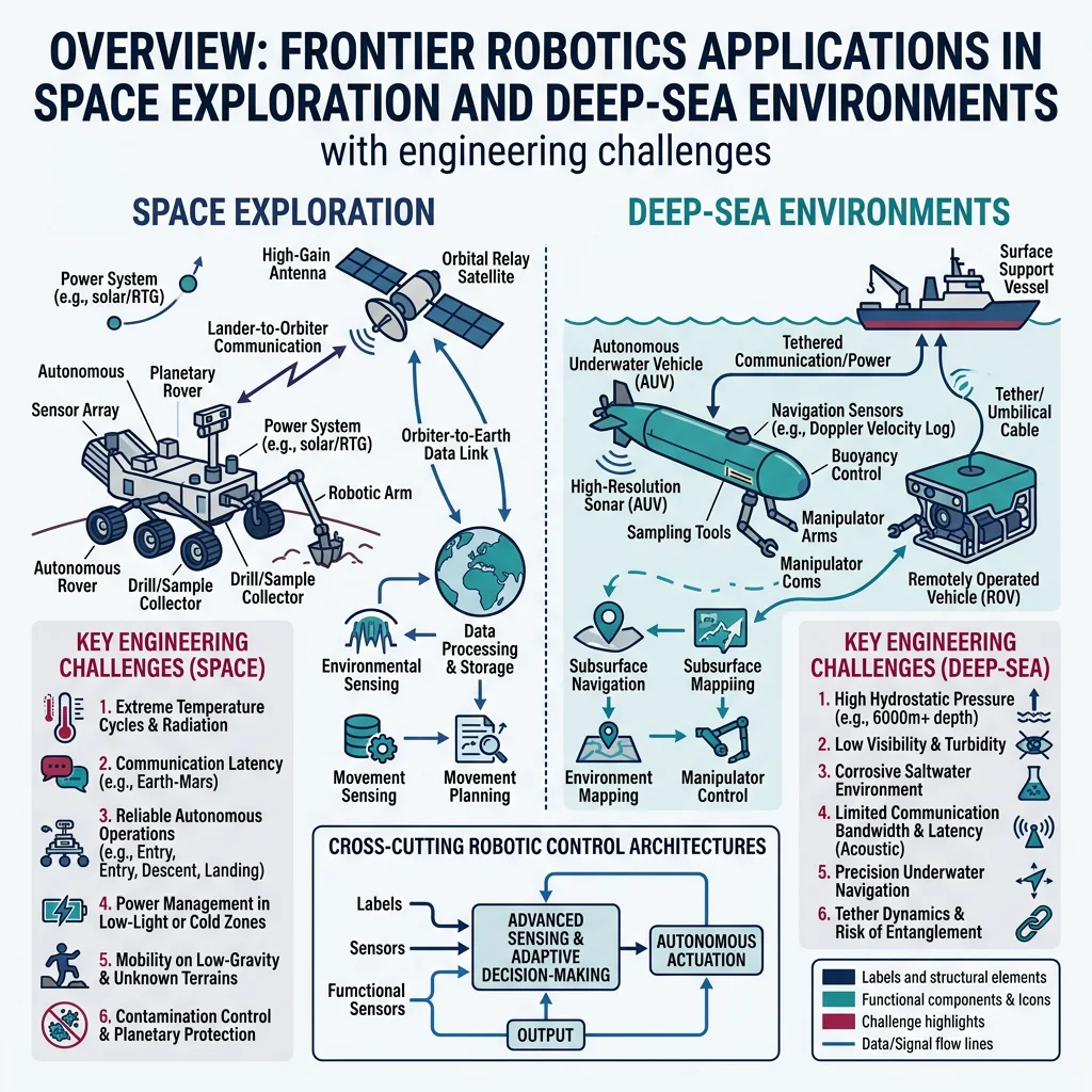
Space & Planetary Robotics

Space robots face extreme challenges: communication delays of up to 24 minutes (Mars), temperature swings of ±200°C, radiation damage, and zero gravity. Every gram of mass costs ~$10,000 to launch to orbit, demanding lightweight, highly reliable designs.

System	Agency	Mission	Key Innovation
Perseverance + Ingenuity	NASA	Mars exploration	First powered flight on another planet
Canadarm2	CSA/NASA	ISS maintenance	17 m arm, inchworm locomotion, 116 ton capacity
OSIRIS-REx	NASA	Asteroid sample return	Touch-and-go sampling from Bennu
GITAI S2	GITAI (Japan)	ISS in-space servicing	Autonomous dexterous manipulation in microgravity
ATHLETE	NASA JPL	Lunar construction	6-legged walking/rolling platform for habitat assembly

import numpy as np
import matplotlib.pyplot as plt

def mars_comms_delay(earth_mars_au):
    """Calculate one-way light travel time to Mars.
    earth_mars_au: distance in astronomical units (AU)
    1 AU = 149,597,870.7 km, light speed = 299,792.458 km/s
    """
    dist_km = earth_mars_au * 149_597_870.7
    return dist_km / 299_792.458  # seconds

# Mars distance varies from 0.37 AU (opposition) to 2.68 AU (conjunction)
distances = np.linspace(0.37, 2.68, 100)
delays = [mars_comms_delay(d) / 60 for d in distances]  # convert to minutes

plt.figure(figsize=(9, 5))
plt.fill_between(distances, delays, alpha=0.2, color='teal')
plt.plot(distances, delays, 'teal', linewidth=2)
plt.axhline(y=mars_comms_delay(0.37)/60, color='g', linestyle='--', label=f'Closest: {mars_comms_delay(0.37)/60:.1f} min')
plt.axhline(y=mars_comms_delay(2.68)/60, color='r', linestyle='--', label=f'Farthest: {mars_comms_delay(2.68)/60:.1f} min')
plt.xlabel('Earth-Mars Distance (AU)')
plt.ylabel('One-Way Light Delay (minutes)')
plt.title('Communication Delay to Mars: Why Rovers Must Be Autonomous')
plt.legend()
plt.grid(True, alpha=0.3)
plt.tight_layout()
plt.show()
print(f"Round-trip at closest approach: {2*mars_comms_delay(0.37)/60:.1f} min")
print(f"Round-trip at farthest: {2*mars_comms_delay(2.68)/60:.1f} min")

Deep-Sea Exploration

The deep ocean is Earth's last frontier — less explored than the surface of Mars. At 11,000 meters depth in the Mariana Trench, pressure reaches 1,100 atmospheres (111 MPa), temperature hovers near 1-4°C, and there is total darkness. Robots designed for this environment must withstand forces that would crush a submarine.

ROV vs. AUV Architectures

Feature	ROV (Remotely Operated)	AUV (Autonomous Underwater)
Power	Tethered (surface ship)	Battery (Li-ion, Li-polymer)
Communication	Fiber-optic tether (real-time)	Acoustic (limited bandwidth)
Depth Rating	Up to 11,000 m (Nereus)	Up to 6,000 m (typical)
Mission Duration	Days (with ship support)	Hours to weeks
Manipulation	Multi-DOF hydraulic arms	Limited (payload samplers)
Best For	Inspection, repair, sampling	Survey, mapping, monitoring

Quantum Sensing & Neuromorphic Computing for Robotics

Two emerging technologies promise to fundamentally transform robot capabilities: quantum sensing for unprecedented measurement precision, and neuromorphic computing for brain-like processing efficiency.

Quantum Sensing

Quantum sensors exploit quantum mechanical phenomena — superposition, entanglement, and interference — to measure physical quantities with sensitivity far beyond classical sensors:

Quantum Sensor	Measures	Sensitivity Gain	Robotics Application
Atom Interferometer	Acceleration, gravity	10–1000×	GPS-denied navigation (inertial)
NV-Center Magnetometer	Magnetic field	fT/√Hz level	Subsurface metal detection, medical imaging
Quantum Gravimeter	Gravitational field gradient	μGal precision	Underground void mapping
Squeezed Light Sensor	Displacement	Below shot noise	Ultra-precise force sensing

Neuromorphic Computing

Traditional processors (von Neumann architecture) shuttle data between memory and CPU — a bottleneck called the "memory wall." The human brain processes information differently: neurons compute and store data in the same structure, using spike-based communication that only consumes energy when information changes. Neuromorphic chips mimic this architecture.

Chip	Developer	Neurons	Synapses	Power	Application
Loihi 2	Intel	1 million	120 million	~1 W	Event-driven perception, SLAM
TrueNorth	IBM	1 million	256 million	~70 mW	Pattern recognition, classification
SpiNNaker 2	U. Manchester	10 million	10 billion	~10 W	Large-scale brain simulation
Akida	BrainChip	1.2 million	10 billion	~300 mW	Edge AI, sensor processing

import numpy as np
import matplotlib.pyplot as plt

def spiking_neuron_lif(I_input, dt=0.001, T=0.1, tau=0.02,
                        V_thresh=-55e-3, V_reset=-70e-3, V_rest=-70e-3,
                        R=10e6):
    """Leaky Integrate-and-Fire (LIF) neuron model.
    Fundamental building block of neuromorphic computing.
    tau * dV/dt = -(V - V_rest) + R * I
    """
    steps = int(T / dt)
    V = np.zeros(steps)
    spikes = []
    V[0] = V_rest

    for t in range(1, steps):
        # Leaky integration
        dV = (-(V[t-1] - V_rest) + R * I_input[t-1]) * dt / tau
        V[t] = V[t-1] + dV

        # Spike and reset
        if V[t] >= V_thresh:
            spikes.append(t * dt)
            V[t] = V_reset

    return V, spikes

# Simulate with different input currents
dt = 0.0001
T = 0.1
t = np.arange(0, T, dt)

fig, axes = plt.subplots(3, 1, figsize=(10, 8), sharex=True)
currents = [2e-9, 4e-9, 8e-9]  # nA
labels = ['2 nA (sub-threshold)', '4 nA (regular spiking)', '8 nA (fast spiking)']

for idx, (I_val, label) in enumerate(zip(currents, labels)):
    I_input = np.ones(len(t)) * I_val
    V, spikes = spiking_neuron_lif(I_input, dt=dt, T=T)
    axes[idx].plot(t * 1000, V * 1000, 'b-', linewidth=1)
    for sp in spikes:
        axes[idx].axvline(x=sp * 1000, color='r', alpha=0.5, linewidth=0.5)
    axes[idx].set_ylabel('V (mV)')
    axes[idx].set_title(f'{label} — {len(spikes)} spikes')
    axes[idx].grid(True, alpha=0.2)

axes[2].set_xlabel('Time (ms)')
plt.suptitle('Leaky Integrate-and-Fire Neuron: Building Block of Neuromorphic Chips', fontsize=13)
plt.tight_layout()
plt.show()
print(f"Spike rates: {[len(spiking_neuron_lif(np.ones(len(t))*I, dt=dt, T=T)[1]) for I in currents]}")

Emerging Tech Research Planner

Use this interactive tool to plan your research or project in any of the advanced robotics domains covered in this article. Capture your focus area, technologies of interest, key challenges, and export as a structured document.

Exercises & Challenges

Conclusion & Next Steps

Advanced and emerging robotics is redefining what robots can be — from rigid machines to soft, adaptive, bio-inspired organisms; from operating rooms to the surface of Mars and the bottom of the ocean. The key takeaways from this exploration:

These technologies are not isolated curiosities — they converge. A future surgical micro-robot might combine soft pneumatic actuation, bio-inspired propulsion, quantum magnetic sensing for navigation, and neuromorphic onboard processing. The engineers who understand these interdisciplinary frontiers will shape the next generation of robotics.