Newton-Euler Formulation
Robotics & Automation Mastery
Introduction to Robotics
History, types, DOF, architectures, mechatronics, ethicsSensors & Perception Systems
Encoders, IMUs, LiDAR, cameras, sensor fusion, Kalman filters, SLAMActuators & Motion Control
DC/servo/stepper motors, hydraulics, drivers, gear systemsKinematics (Forward & Inverse)
DH parameters, transformations, Jacobians, workspace analysisDynamics & Robot Modeling
Newton-Euler, Lagrangian, inertia, friction, contact modelingControl Systems & PID
PID tuning, state-space, LQR, MPC, adaptive & robust controlEmbedded Systems & Microcontrollers
Arduino, STM32, RTOS, PWM, serial protocols, FPGARobot Operating Systems (ROS)
ROS2, nodes, topics, Gazebo, URDF, navigation stacksComputer Vision for Robotics
Calibration, stereo vision, object recognition, visual SLAMAI Integration & Autonomous Systems
ML, reinforcement learning, path planning, swarm roboticsHuman-Robot Interaction (HRI)
Cobots, gesture/voice control, safety standards, social roboticsIndustrial Robotics & Automation
PLC, SCADA, Industry 4.0, smart factories, digital twinsMobile Robotics
Wheeled/legged robots, autonomous vehicles, drones, marine roboticsSafety, Reliability & Compliance
Functional safety, redundancy, ISO standards, cybersecurityAdvanced & Emerging Robotics
Soft robotics, bio-inspired, surgical, space, nano-roboticsSystems Integration & Deployment
HW/SW co-design, testing, field deployment, lifecycleRobotics Business & Strategy
Startups, product-market fit, manufacturing, go-to-marketComplete Robotics System Project
Autonomous rover, pick-and-place arm, delivery robot, swarm simWhile kinematics describes where a robot moves, dynamics describes how it moves — accounting for masses, inertias, gravity, and forces. The Newton-Euler formulation approaches dynamics from first principles: Newton's second law (F = ma) for linear motion and Euler's equation (τ = Iα) for rotational motion.
Forward vs. Inverse Dynamics
| Problem | Given | Find | Use Case |
|---|---|---|---|
| Forward Dynamics | Joint torques τ | Joint accelerations q̈ | Simulation — "apply these torques, how does the robot move?" |
| Inverse Dynamics | Desired trajectory (q, q̇, q̈) | Required torques τ | Control — "what torques produce this motion?" |
Free Body Diagrams for Robot Links
For each link in a robot chain, we draw a free body diagram showing all forces and torques acting on it. The Newton-Euler approach propagates these forces and torques along the chain in two passes:
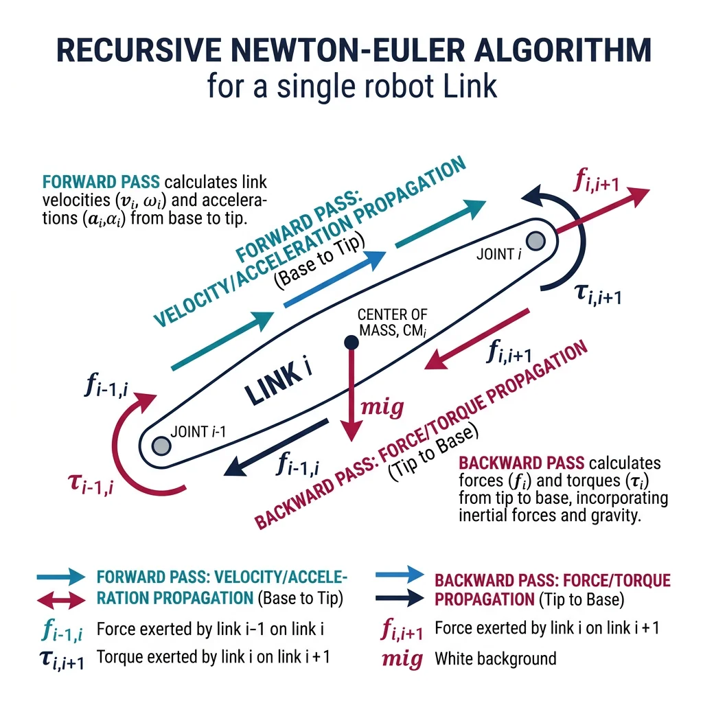
Forward pass (base → tip): Propagate velocities and accelerations from base to end-effector.
Backward pass (tip → base): Propagate forces and torques from end-effector back to base.
import numpy as np

class Link:
    """Represents a single robot link for dynamics computation."""
    def __init__(self, mass, length, inertia, com_offset=0.5):
        self.mass = mass          # kg
        self.length = length      # m
        self.inertia = inertia    # kg·m² (about center of mass)
        self.com = com_offset * length  # center of mass distance from joint

def inverse_dynamics_2link(links, theta, theta_dot, theta_ddot, gravity=9.81):
    """Inverse dynamics for a 2-link planar arm using Newton-Euler.

    Args:
        links: List of Link objects [link1, link2]
        theta: Joint angles [theta1, theta2] in radians
        theta_dot: Joint velocities [w1, w2]
        theta_ddot: Joint accelerations [a1, a2]
        gravity: Gravitational acceleration
    Returns:
        Required joint torques [tau1, tau2]
    """
    m1, m2 = links[0].mass, links[1].mass
    L1, L2 = links[0].length, links[1].length
    lc1, lc2 = links[0].com, links[1].com
    I1, I2 = links[0].inertia, links[1].inertia
    g = gravity

    t1, t2 = theta
    w1, w2 = theta_dot
    a1, a2 = theta_ddot

    # Inertia matrix M(q) — 2x2 for 2-link arm
    M11 = (m1*lc1**2 + I1 + m2*(L1**2 + lc2**2 + 2*L1*lc2*np.cos(t2)) + I2)
    M12 = m2*(lc2**2 + L1*lc2*np.cos(t2)) + I2
    M21 = M12
    M22 = m2*lc2**2 + I2

    # Coriolis/centrifugal terms C(q, q_dot)
    h = -m2 * L1 * lc2 * np.sin(t2)
    C1 = h * (2*w1*w2 + w2**2)  # Coriolis + centrifugal
    C2 = -h * w1**2              # Back-reaction

    # Gravity terms G(q)
    G1 = (m1*lc1 + m2*L1)*g*np.cos(t1) + m2*lc2*g*np.cos(t1 + t2)
    G2 = m2*lc2*g*np.cos(t1 + t2)

    # τ = M(q)·q̈ + C(q,q̇) + G(q)
    tau1 = M11*a1 + M12*a2 + C1 + G1
    tau2 = M21*a1 + M22*a2 + C2 + G2

    return np.array([tau1, tau2])

# Define robot links
link1 = Link(mass=5.0, length=0.5, inertia=0.1)
link2 = Link(mass=3.0, length=0.4, inertia=0.05)

# Scenario: Holding still at 45°, 30° (gravity compensation)
theta = np.radians([45, 30])
tau_static = inverse_dynamics_2link(
    [link1, link2], theta,
    theta_dot=[0, 0], theta_ddot=[0, 0]
)
print("Static Gravity Compensation:")
print(f"  θ = (45°, 30°)")
print(f"  τ1 = {tau_static[0]:.3f} Nm, τ2 = {tau_static[1]:.3f} Nm")

# Scenario: Moving with constant velocity (Coriolis/centrifugal)
tau_moving = inverse_dynamics_2link(
    [link1, link2], theta,
    theta_dot=[1.0, 0.5], theta_ddot=[0, 0]
)
print(f"\nConstant Velocity (ω1=1, ω2=0.5 rad/s):")
print(f"  τ1 = {tau_moving[0]:.3f} Nm, τ2 = {tau_moving[1]:.3f} Nm")

# Scenario: Accelerating (full dynamics)
tau_accel = inverse_dynamics_2link(
    [link1, link2], theta,
    theta_dot=[1.0, 0.5], theta_ddot=[2.0, 1.5]
)
print(f"\nAccelerating (α1=2, α2=1.5 rad/s²):")
print(f"  τ1 = {tau_accel[0]:.3f} Nm, τ2 = {tau_accel[1]:.3f} Nm")
Practical Examples
Case Study: ABB IRB 6700 — Payload Capacity from Dynamics
The ABB IRB 6700 can handle 150 kg with a 3.2m reach. Its datasheet specifies maximum payload, but how is this number determined? Through inverse dynamics analysis.
Process: Engineers model each of the 6 links with mass, inertia tensor, and center of mass. For the worst-case trajectory (maximum acceleration at full extension), they compute the required joint torques via inverse dynamics. The payload limit is where any motor's required torque reaches its peak continuous rating.
Key Insight: Payload capacity depends on the trajectory! A robot can handle more weight when moving slowly near its base than when making fast, extended motions. Dynamics makes this trade-off quantifiable.
Lagrangian Dynamics
The Lagrangian formulation offers an alternative to Newton-Euler that's more elegant for complex systems. Instead of tracking forces on each link, it works with energy — the difference between kinetic and potential energy of the entire system.
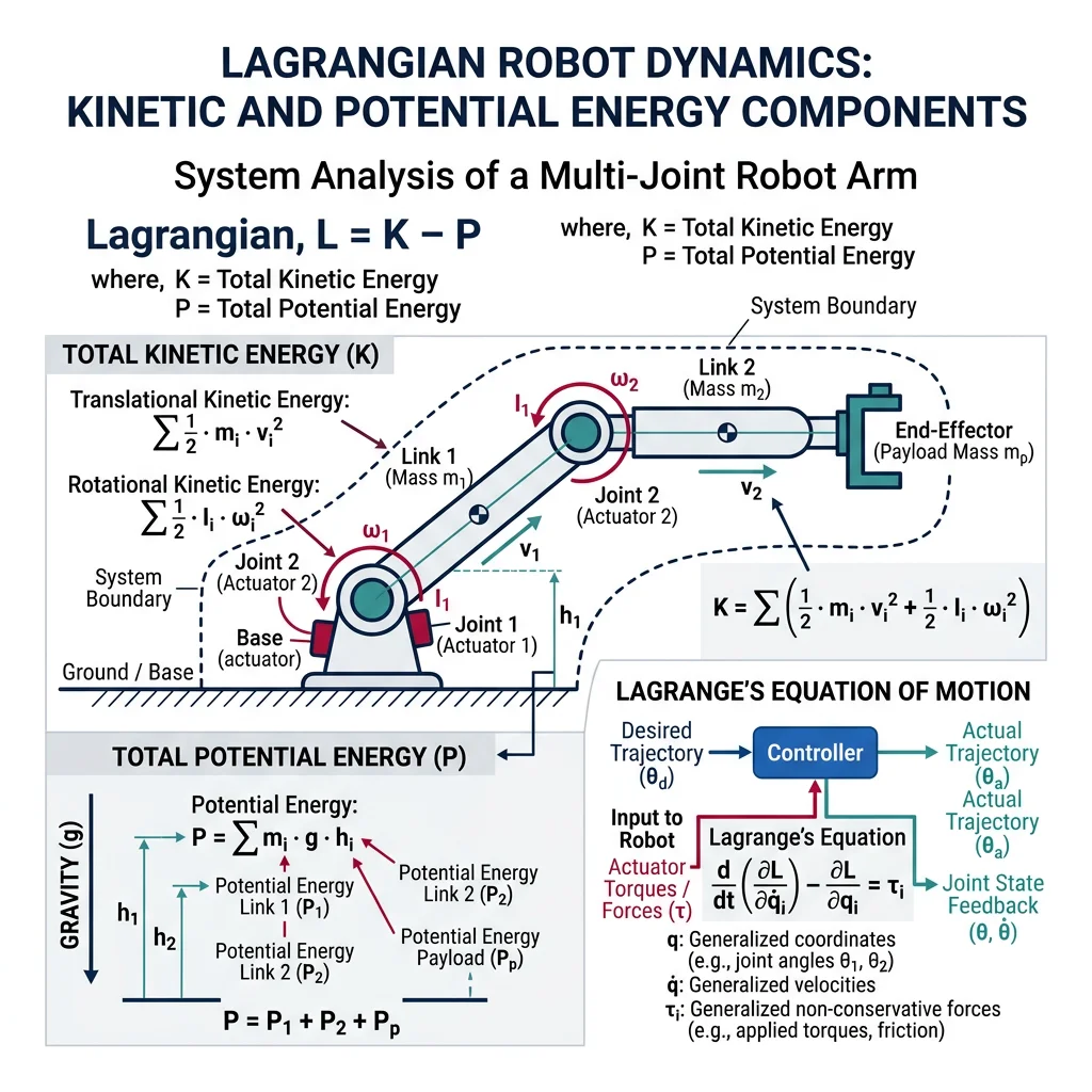
• Newton-Euler is computationally efficient (O(n) for n joints) — ideal for real-time control
• Lagrangian is mathematically elegant and gives the equations of motion in closed form — ideal for analysis and design
L = T − V (Lagrangian = Kinetic Energy − Potential Energy)
d/dt(∂L/∂q̇ᵢ) − ∂L/∂qᵢ = τᵢ (Euler-Lagrange equation for joint i)
import numpy as np

def lagrangian_1link(theta, theta_dot, theta_ddot,
                     mass=2.0, length=0.5, gravity=9.81):
    """Lagrangian dynamics for a single pendulum (1-link arm).

    The simplest possible example to illustrate the method.
    Kinetic energy: T = 0.5 * I * theta_dot^2
    Potential energy: V = m * g * lc * cos(theta)
    """
    lc = length / 2  # Center of mass at link midpoint
    I = mass * lc**2  # Simplified inertia (point mass approximation)

    # Energy components
    T = 0.5 * I * theta_dot**2
    V = mass * gravity * lc * np.cos(theta)
    L = T - V

    # Euler-Lagrange equation: I*theta_ddot + m*g*lc*sin(theta) = tau
    tau = I * theta_ddot + mass * gravity * lc * np.sin(theta)

    return tau, T, V

# Example: gravity torque at different angles
print("1-Link Arm (Pendulum) — Lagrangian Dynamics")
print(f"Mass=2.0kg, Length=0.5m")
print("=" * 55)

angles = [0, 30, 45, 90, 180]
for deg in angles:
    rad = np.radians(deg)
    tau, T, V = lagrangian_1link(rad, 0, 0)
    print(f"θ={deg:4d}° → τ_gravity={tau:7.3f} Nm, "
          f"T={T:.3f} J, V={V:7.3f} J")

# With motion: accelerating at 5 rad/s² from 45°
tau_accel, T, V = lagrangian_1link(np.radians(45), 2.0, 5.0)
print(f"\nθ=45°, ω=2 rad/s, α=5 rad/s²:")
print(f"  Required torque: {tau_accel:.3f} Nm")
print(f"  (gravity component: {2.0*9.81*0.25*np.sin(np.radians(45)):.3f} Nm)")
print(f"  (inertial component: {2.0*0.25**2 * 5.0:.3f} Nm)")
Mass & Inertia Matrices
For multi-link robots, the dynamics equation takes the elegant matrix form:
τ = M(q)·q̈ + C(q, q̇)·q̇ + G(q)
Where:
• M(q) — Mass/inertia matrix (n×n, symmetric, positive definite)
• C(q, q̇) — Coriolis and centrifugal matrix
• G(q) — Gravity vector
• q, q̇, q̈ — Joint positions, velocities, accelerations
• τ — Joint torques
import numpy as np

def compute_dynamics_matrices(theta, m1=5.0, m2=3.0,
                               L1=0.5, L2=0.4, g=9.81):
    """Compute M, C, G matrices for a 2-link planar arm.

    Returns the three fundamental dynamics matrices.
    """
    lc1, lc2 = L1/2, L2/2
    I1 = m1 * L1**2 / 12  # Rod inertia about center
    I2 = m2 * L2**2 / 12

    t2 = theta[1]

    # Mass matrix M(q)
    M = np.array([
        [m1*lc1**2 + I1 + m2*(L1**2 + lc2**2 + 2*L1*lc2*np.cos(t2)) + I2,
         m2*(lc2**2 + L1*lc2*np.cos(t2)) + I2],
        [m2*(lc2**2 + L1*lc2*np.cos(t2)) + I2,
         m2*lc2**2 + I2]
    ])

    # Coriolis matrix C(q, q_dot) using Christoffel symbols
    h = m2 * L1 * lc2 * np.sin(t2)
    C = np.array([
        [-h, -h],
        [ h,  0]
    ])

    # Gravity vector G(q)
    G = np.array([
        (m1*lc1 + m2*L1)*g*np.cos(theta[0]) + m2*lc2*g*np.cos(theta[0]+t2),
        m2*lc2*g*np.cos(theta[0] + t2)
    ])

    return M, C, G

# Analyze dynamics at different configurations
configs = [
    (np.radians([0, 0]), "Horizontal, extended"),
    (np.radians([90, 0]), "Vertical, extended"),
    (np.radians([0, 90]), "Horizontal, elbow bent"),
]

for theta, desc in configs:
    M, C, G = compute_dynamics_matrices(theta)
    print(f"\nConfiguration: {desc}")
    print(f"  M (mass matrix):\n    {np.round(M, 4)}")
    print(f"  det(M) = {np.linalg.det(M):.6f} (always > 0)")
    print(f"  G (gravity): [{G[0]:.3f}, {G[1]:.3f}] Nm")

    # Eigenvalues of M show principal inertias
    eigvals = np.linalg.eigvals(M)
    print(f"  Principal inertias: {np.round(eigvals, 4)}")
    print(f"  Condition number: {max(eigvals)/min(eigvals):.2f}")
1. Symmetric: M = MT (always)
2. Positive Definite: xTMx > 0 for all x ≠ 0 (kinetic energy is always positive)
3. Configuration-Dependent: M changes as the robot moves
4. Bounded: λmin(M) ≤ ||M|| ≤ λmax(M) — important for control stability
Friction & Contact Modeling
Real robots aren't frictionless. Friction in joints, gears, and bearings significantly affects performance. Accurate friction models are critical for precise control, especially at low speeds.
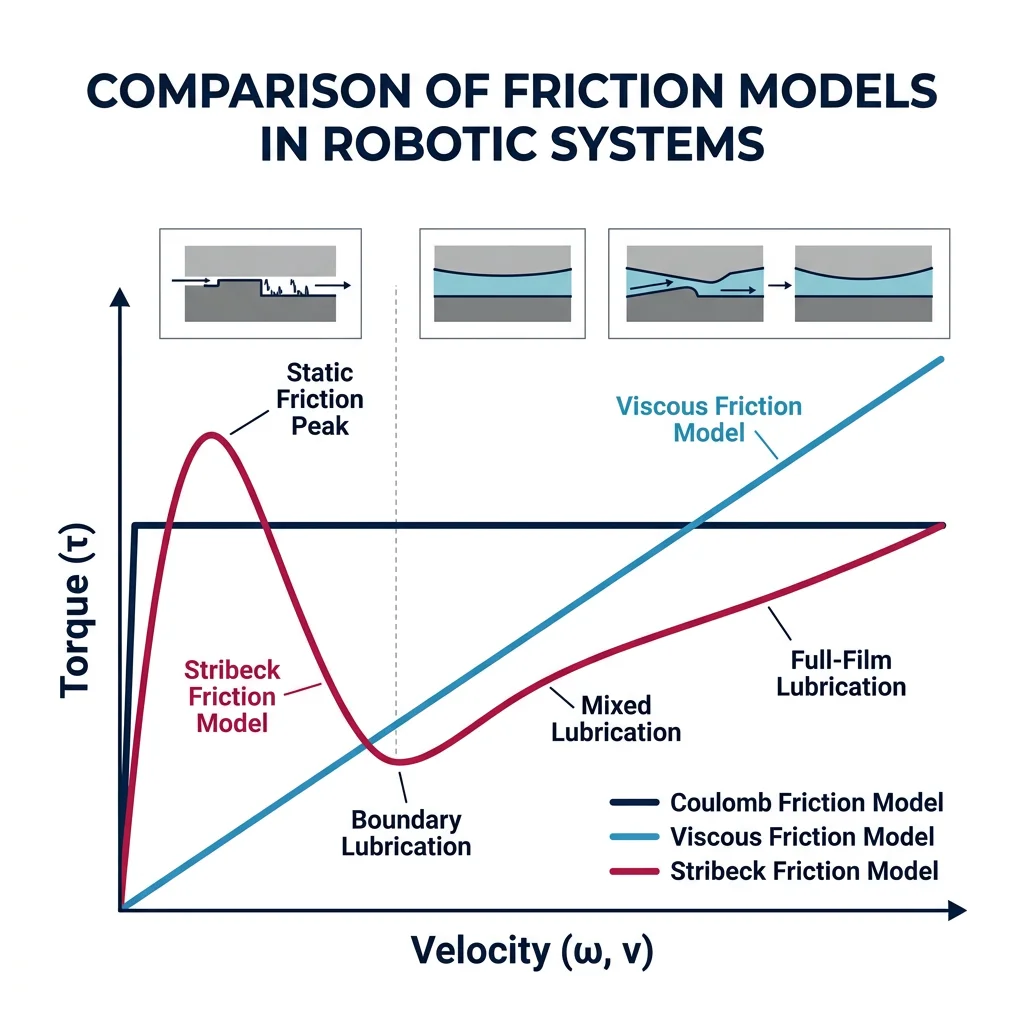
Friction Models
| Model | Equation | Captures | Complexity |
|---|---|---|---|
| Coulomb | τ_f = μ·sign(q̇) | Constant kinetic friction | Simple |
| Viscous | τ_f = b·q̇ | Velocity-dependent damping | Simple |
| Coulomb + Viscous | τ_f = μ·sign(q̇) + b·q̇ | Both effects combined | Moderate |
| Stribeck | τ_f includes velocity-dependent static→kinetic transition | Stick-slip at low speeds | Complex |
| LuGre | State-dependent bristle model | Pre-sliding, hysteresis | Advanced |
import numpy as np

def coulomb_friction(velocity, mu=0.5):
    """Coulomb (dry) friction — constant magnitude, opposes motion."""
    return mu * np.sign(velocity)

def viscous_friction(velocity, b=0.1):
    """Viscous (fluid) friction — proportional to velocity."""
    return b * velocity

def combined_friction(velocity, mu=0.5, b=0.1):
    """Coulomb + viscous friction model."""
    return mu * np.sign(velocity) + b * velocity

def stribeck_friction(velocity, mu_s=0.8, mu_k=0.5, b=0.1, v_s=0.1):
    """Stribeck friction model — captures stick-slip behavior.

    Args:
        mu_s: Static friction coefficient
        mu_k: Kinetic friction coefficient
        b: Viscous coefficient
        v_s: Stribeck velocity (transition speed)
    """
    # Stribeck curve: smooth transition from static to kinetic
    stribeck = mu_k + (mu_s - mu_k) * np.exp(-(velocity / v_s)**2)
    return stribeck * np.sign(velocity) + b * velocity

# Compare friction models
velocities = np.linspace(-2, 2, 201)

print("Friction Model Comparison at v = 0.5 rad/s")
print("=" * 50)
v_test = 0.5
print(f"Coulomb:   Ï" = {coulomb_friction(v_test):.3f} Nm")
print(f"Viscous:   Ï" = {viscous_friction(v_test):.3f} Nm")
print(f"Combined:  Ï" = {combined_friction(v_test):.3f} Nm")
print(f"Stribeck:  Ï" = {stribeck_friction(v_test):.3f} Nm")

# Show Stribeck effect at low speeds
print(f"\nStribeck Effect at Low Speeds:")
for v in [0.01, 0.05, 0.1, 0.5, 1.0]:
    f_strib = stribeck_friction(v)
    f_comb = combined_friction(v)
    print(f"  v={v:.2f}: Stribeck={f_strib:.3f}, Combined={f_comb:.3f}")
Contact Dynamics
When robots interact with the environment — grasping objects, walking on ground, or doing assembly — contact dynamics become essential. Contacts introduce discontinuities (impact) and constraints (non-penetration).
Case Study: Boston Dynamics Spot — Contact-Rich Locomotion
Boston Dynamics' Spot robot navigates rough terrain by continuously making and breaking contact with the ground through its 12 actuated joints (3 per leg). Each footfall involves:
Impact dynamics: When a foot strikes the ground, the robot experiences an impulsive force transfer. Spot's controller must predict and compensate for these impacts in real time.
Friction cone constraints: Each foot contact is stable only if the ground reaction force stays within the friction cone (no slipping). Spot continuously monitors this to determine safe footholds.
Contact scheduling: The gait planner decides which feet are in contact and when — balancing stability, speed, and energy efficiency. This is a hybrid dynamics problem (continuous motion + discrete contact events).
import numpy as np

def spring_damper_contact(penetration, velocity,
                          k=10000, b=500, mu=0.5):
    """Simple spring-damper contact model.

    Models ground contact as a spring + damper when penetration > 0.
    Friction modeled with Coulomb model.

    Args:
        penetration: Depth below ground (positive = contact)
        velocity: [vx, vz] velocity at contact point
        k: Contact stiffness (N/m)
        b: Contact damping (N·s/m)
        mu: Friction coefficient
    Returns:
        Contact force [Fx, Fz]
    """
    if penetration <= 0:
        return np.array([0.0, 0.0])  # No contact

    # Normal force (spring-damper, only compressive)
    Fn = k * penetration - b * velocity[1]
    Fn = max(Fn, 0)  # Can only push, not pull

    # Tangential friction force
    Ft = -mu * Fn * np.sign(velocity[0]) if abs(velocity[0]) > 1e-6 else 0

    return np.array([Ft, Fn])

# Simulate a ball dropping onto ground
print("Spring-Damper Contact Model Simulation")
print("=" * 50)

# Ball parameters
mass = 1.0  # kg
z = 0.5     # initial height (m)
vz = 0.0    # initial vertical velocity
vx = 0.2    # horizontal velocity
dt = 0.001  # time step
g = 9.81

print(f"Ball: mass={mass}kg, initial height={z}m")
print(f"Contact: k=10000 N/m, b=500 N·s/m, μ=0.5")
print(f"\nTime    Height   Velocity  Contact Force")
print("-" * 50)

for step in range(500):
    t = step * dt
    penetration = -z  # Positive when below ground (z=0)
    F = spring_damper_contact(penetration, np.array([vx, vz]))

    # Update dynamics: a = F/m - g
    az = F[1]/mass - g
    ax = F[0]/mass

    vz += az * dt
    vx += ax * dt
    z += vz * dt

    if step % 50 == 0:
        print(f"{t:.3f}s  {z:8.4f}m  {vz:8.4f} m/s  Fz={F[1]:8.1f} N")
Advanced Dynamics Topics
Manipulator Dynamics
Industrial manipulators present unique dynamics challenges due to their serial structure, high gear ratios, and need for precision. Key considerations include:
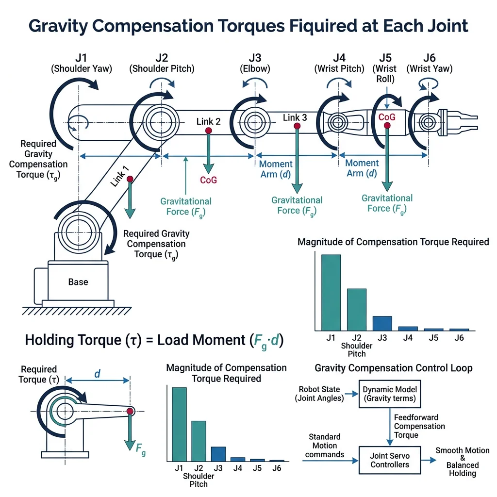
Gravity Compensation
Many industrial robots dedicate significant motor torque just to fighting gravity. Gravity compensation pre-computes the gravity torque G(q) and feeds it forward, freeing the controller to focus on motion control.
import numpy as np

def gravity_compensation(theta, m1=5.0, m2=3.0,
                          L1=0.5, L2=0.4, g=9.81):
    """Compute gravity compensation torques for a 2-link arm.

    These torques exactly cancel gravity at the given configuration.
    """
    lc1, lc2 = L1/2, L2/2

    G1 = (m1*lc1 + m2*L1)*g*np.cos(theta[0]) + m2*lc2*g*np.cos(theta[0]+theta[1])
    G2 = m2*lc2*g*np.cos(theta[0] + theta[1])

    return np.array([G1, G2])

# Show gravity torques across workspace
print("Gravity Compensation Torques Across Configurations")
print("=" * 55)
print("2-Link arm: m1=5kg, m2=3kg, L1=0.5m, L2=0.4m")
print(f"{'θ1':>6} {'θ2':>6} {'τ1_grav':>10} {'τ2_grav':>10} {'Total':>10}")
print("-" * 55)

for t1 in [0, 30, 45, 60, 90]:
    for t2 in [0, 45, 90]:
        theta = np.radians([t1, t2])
        G = gravity_compensation(theta)
        print(f"{t1:6d}° {t2:6d}° {G[0]:10.3f} {G[1]:10.3f} "
              f"{np.sum(np.abs(G)):10.3f} Nm")

# Key insight: maximum gravity torque at horizontal
theta_max = np.radians([0, 0])
G_max = gravity_compensation(theta_max)
print(f"\nMax gravity load (arm horizontal): τ1={G_max[0]:.3f} Nm")
print(f"This requires {G_max[0]:.1f} Nm continuous torque just to hold position!")
Mobile Robot Dynamics
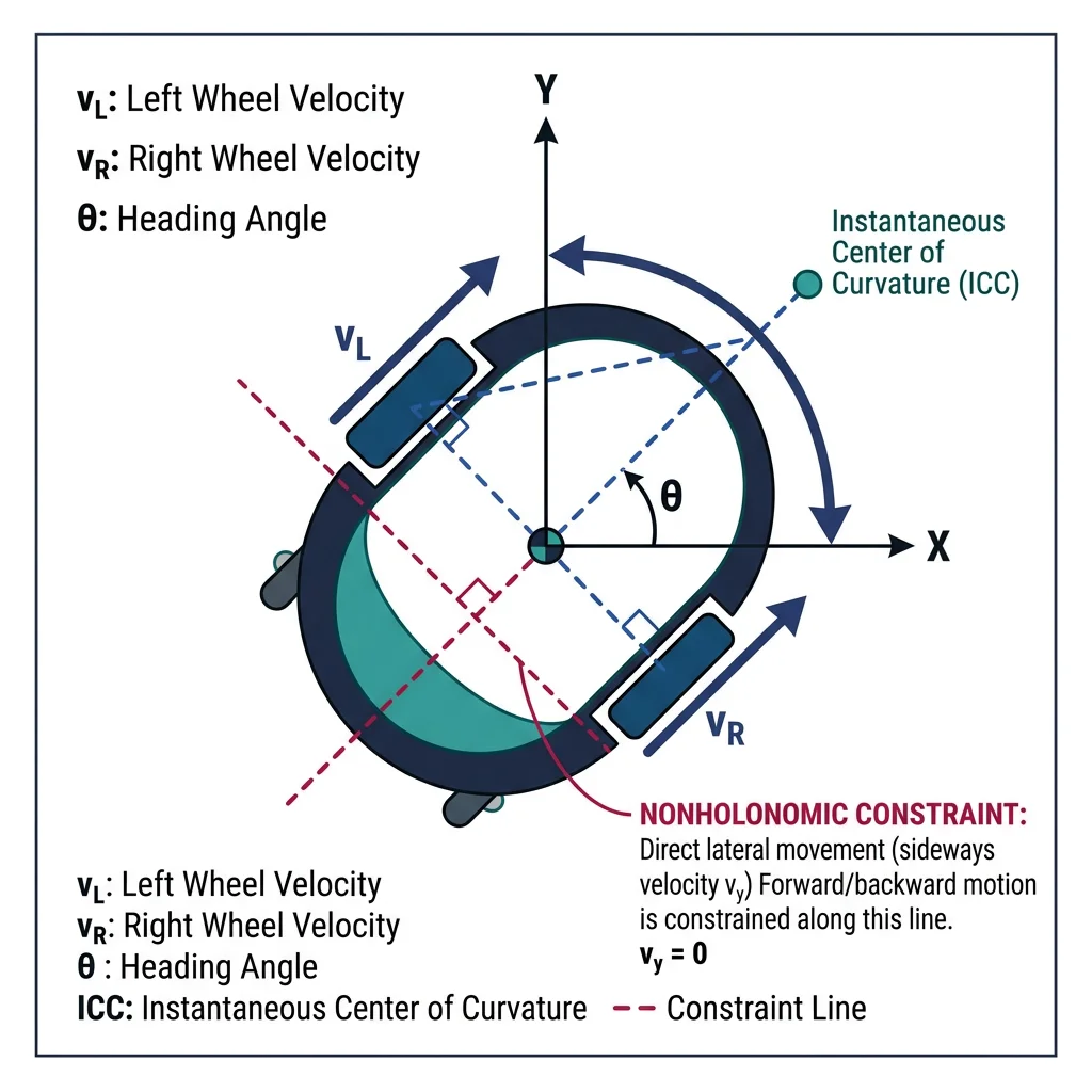
Mobile robots have fundamentally different dynamics from manipulators. They move through space under nonholonomic constraints — restrictions on velocity that cannot be integrated into position constraints.
import numpy as np

def differential_drive_dynamics(state, v_left, v_right,
                                  wheel_radius=0.05, wheel_base=0.3, dt=0.01):
    """Simulate differential drive robot dynamics.

    State: [x, y, theta] — position and heading
    Inputs: left and right wheel velocities (rad/s)
    """
    x, y, theta = state
    R = wheel_radius
    L = wheel_base

    # Convert wheel velocities to robot velocities
    v = R * (v_right + v_left) / 2       # Linear velocity
    omega = R * (v_right - v_left) / L    # Angular velocity

    # Update state (Euler integration)
    x_new = x + v * np.cos(theta) * dt
    y_new = y + v * np.sin(theta) * dt
    theta_new = theta + omega * dt

    return np.array([x_new, y_new, theta_new]), v, omega

# Simulate different motions
state = np.array([0.0, 0.0, 0.0])  # Start at origin facing +X
dt = 0.01

print("Differential Drive Robot Dynamics")
print("=" * 55)

# Motion 1: Straight line
print("\n1. Straight Line (both wheels same speed):")
s = np.array([0.0, 0.0, 0.0])
for _ in range(100):
    s, v, w = differential_drive_dynamics(s, 10.0, 10.0, dt=dt)
print(f"   After 1s: x={s[0]:.3f}, y={s[1]:.3f}, θ={np.degrees(s[2]):.1f}°")

# Motion 2: Pure rotation (spin in place)
print("\n2. Pure Rotation (wheels opposite speeds):")
s = np.array([0.0, 0.0, 0.0])
for _ in range(100):
    s, v, w = differential_drive_dynamics(s, -10.0, 10.0, dt=dt)
print(f"   After 1s: x={s[0]:.4f}, y={s[1]:.4f}, θ={np.degrees(s[2]):.1f}°")

# Motion 3: Arc turn
print("\n3. Arc Turn (different wheel speeds):")
s = np.array([0.0, 0.0, 0.0])
for _ in range(300):
    s, v, w = differential_drive_dynamics(s, 8.0, 12.0, dt=dt)
print(f"   After 3s: x={s[0]:.3f}, y={s[1]:.3f}, θ={np.degrees(s[2]):.1f}°")
print(f"   Turn radius: {0.05*(12+8)/(2*(12-8)/0.3):.3f} m")
Energy-Based Modeling
Energy methods provide powerful tools for analyzing robot dynamics without solving differential equations directly.
• Kinetic Energy: T = ½ q̇T M(q) q̇ — always positive, depends on velocities and configuration
• Potential Energy: V = Σ mᵢ g hᵢ — gravitational potential of each link
• Power: P = τT q̇ — rate of energy input from motors
• Passivity: The decrease in stored energy ≤ power input (fundamental for stable control)
import numpy as np

def compute_energy(theta, theta_dot, m1=5.0, m2=3.0,
                   L1=0.5, L2=0.4, g=9.81):
    """Compute kinetic and potential energy for a 2-link arm."""
    lc1, lc2 = L1/2, L2/2
    I1, I2 = m1*L1**2/12, m2*L2**2/12
    t1, t2 = theta
    w1, w2 = theta_dot

    # Heights of centers of mass
    h1 = lc1 * np.sin(t1)
    h2 = L1 * np.sin(t1) + lc2 * np.sin(t1 + t2)

    # Potential energy
    V = m1*g*h1 + m2*g*h2

    # Kinetic energy (from mass matrix)
    M11 = m1*lc1**2 + I1 + m2*(L1**2 + lc2**2 + 2*L1*lc2*np.cos(t2)) + I2
    M12 = m2*(lc2**2 + L1*lc2*np.cos(t2)) + I2
    M22 = m2*lc2**2 + I2

    T = 0.5 * (M11*w1**2 + 2*M12*w1*w2 + M22*w2**2)

    return T, V, T + V

# Energy analysis along a trajectory
print("Energy Analysis — 2-Link Arm Swinging Under Gravity")
print("=" * 60)
print(f"{'Angle':>8} {'Kinetic':>10} {'Potential':>10} {'Total':>10}")
print("-" * 60)

# Simulate pendulum-like swing (no motors, gravity only)
t1, t2 = np.radians(60), np.radians(0)
w1, w2 = 0.0, 0.0
dt = 0.01

for step in range(500):
    T, V, E = compute_energy([t1, t2], [w1, w2])

    if step % 50 == 0:
        print(f"{np.degrees(t1):8.1f}° {T:10.3f} J {V:10.3f} J {E:10.3f} J")

    # Simple gravity-driven update (no friction)
    lc1 = 0.25
    alpha1 = -(5.0*lc1 + 3.0*0.5)*9.81*np.cos(t1) / (5.0*lc1**2 + 3.0*0.5**2 + 5.0*0.5**2/12)
    w1 += alpha1 * dt
    t1 += w1 * dt

print(f"\nNote: Total energy should remain approximately constant")
print(f"(conservation of energy — no friction or external forces)")
Dynamics Parameter Calculator
Use this tool to document your robot's dynamic parameters and compute key quantities. Enter link masses, lengths, and inertias, then download as Word, Excel, or PDF.
Dynamics Parameter Calculator
Enter link physical properties. Format: mass(kg), length(m), inertia(kg·m²) per link. Download as Word, Excel, or PDF.
All data stays in your browser. Nothing is sent to or stored on any server.
Exercises & Challenges
Exercise 1: Gravity Torque Computation
Compute the gravity compensation torques for a 2-link arm at θ = (0°, 0°) — the worst case. Then compare with θ = (90°, 0°) — the arm pointing straight up.
import numpy as np

def gravity_torques(t1_deg, t2_deg, m1=5.0, m2=3.0, L1=0.5, L2=0.4, g=9.81):
    t1, t2 = np.radians(t1_deg), np.radians(t2_deg)
    lc1, lc2 = L1/2, L2/2
    G1 = (m1*lc1 + m2*L1)*g*np.cos(t1) + m2*lc2*g*np.cos(t1+t2)
    G2 = m2*lc2*g*np.cos(t1 + t2)
    return G1, G2

# Worst case: horizontal
G1, G2 = gravity_torques(0, 0)
print(f"Horizontal (0°, 0°): τ1={G1:.3f} Nm, τ2={G2:.3f} Nm")

# Best case: vertical
G1, G2 = gravity_torques(90, 0)
print(f"Vertical (90°, 0°): τ1={G1:.3f} Nm, τ2={G2:.3f} Nm")

print(f"\n→ Gravity torque drops to near zero when arm points up!")
Exercise 2: Inverse Dynamics for a Trajectory
Compute the required torques for a 1-link arm to track a sinusoidal trajectory: θ(t) = 45° · sin(2πt). What are the peak torques?
import numpy as np

mass, length, g = 3.0, 0.4, 9.81
lc = length / 2
I = mass * length**2 / 12

t = np.linspace(0, 1, 101)
amplitude = np.radians(45)
omega = 2 * np.pi  # 1 Hz

theta = amplitude * np.sin(omega * t)
theta_dot = amplitude * omega * np.cos(omega * t)
theta_ddot = -amplitude * omega**2 * np.sin(omega * t)

# Inverse dynamics: tau = I*alpha + m*g*lc*sin(theta)
tau = (mass*lc**2 + I) * theta_ddot + mass*g*lc*np.sin(theta)

print("Sinusoidal Trajectory Inverse Dynamics")
print(f"θ(t) = 45°·sin(2πt), mass={mass}kg, L={length}m")
print(f"Peak θ_ddot = {np.max(np.abs(theta_ddot)):.2f} rad/s²")
print(f"Peak torque = {np.max(np.abs(tau)):.3f} Nm")
print(f"Inertial peak = {np.max(np.abs((mass*lc**2+I)*theta_ddot)):.3f} Nm")
print(f"Gravity peak  = {mass*g*lc:.3f} Nm")
Exercise 3: Friction Identification
Given velocity-torque measurements from a motor, identify the Coulomb and viscous friction parameters using curve fitting.
import numpy as np

# Simulated measurements (with noise)
np.random.seed(42)
true_mu, true_b = 0.4, 0.08
velocities = np.array([0.5, 1.0, 1.5, 2.0, 3.0, 4.0, 5.0])
torques = true_mu + true_b * velocities + np.random.normal(0, 0.02, len(velocities))

# Linear regression: tau = mu + b*v → [1, v] @ [mu, b]^T = tau
A = np.column_stack([np.ones_like(velocities), velocities])
params, _, _, _ = np.linalg.lstsq(A, torques, rcond=None)
mu_est, b_est = params

print("Friction Parameter Identification")
print(f"True:      μ={true_mu:.3f} Nm, b={true_b:.4f} Nm·s/rad")
print(f"Estimated: μ={mu_est:.3f} Nm, b={b_est:.4f} Nm·s/rad")
print(f"Error:     μ_err={abs(mu_est-true_mu):.4f}, b_err={abs(b_est-true_b):.5f}")
Conclusion & Next Steps
In this article, we've explored the physics that governs robot motion:
- Newton-Euler formulation provides an efficient recursive algorithm (O(n)) for computing joint torques
- Lagrangian dynamics derives elegant closed-form equations of motion using energy methods
- The robot equation τ = M(q)q̈ + C(q,q̇)q̇ + G(q) captures all dynamic effects in matrix form
- Friction models (Coulomb, viscous, Stribeck) account for real-world joint resistance
- Contact dynamics handle robot-environment interaction essential for manipulation and locomotion
- Energy methods provide powerful analysis tools and the foundation for stability-guaranteed control