Introduction
CPU pipelining is a fundamental technique that allows processors to execute multiple instructions simultaneously by overlapping their execution stages. Understanding pipelining reveals how modern CPUs achieve high throughput despite instruction-level dependencies.
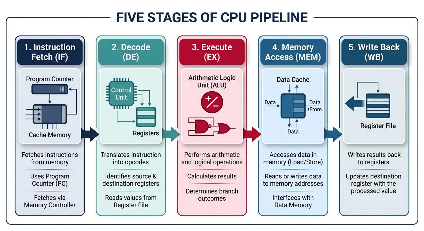
Series Context: This is Part 7 of 24 in the Computer Architecture & Operating Systems Mastery series. Building on compilers and program translation, we now explore how CPUs execute instructions efficiently through pipelining.
1
Part 1: Foundations of Computer Systems
System overview, architectures, OS role
2
Digital Logic & CPU Building Blocks
Gates, registers, datapath, microarchitecture
3
Instruction Set Architecture (ISA)
RISC vs CISC, instruction formats, addressing
4
Assembly Language & Machine Code
Registers, stack, calling conventions
5
Assemblers, Linkers & Loaders
Object files, ELF, dynamic linking
6
Compilers & Program Translation
Lexing, parsing, code generation
7
CPU Execution & Pipelining
Fetch-decode-execute, hazards, prediction
You Are Here
8
OS Architecture & Kernel Design
Monolithic, microkernel, system calls
9
Processes & Program Execution
Process lifecycle, PCB, fork/exec
10
Threads & Concurrency
Threading models, pthreads, race conditions
11
CPU Scheduling Algorithms
FCFS, RR, CFS, real-time scheduling
12
Synchronization & Coordination
Locks, semaphores, classic problems
13
Deadlocks & Prevention
Coffman conditions, Banker's algorithm
14
Memory Hierarchy & Cache
L1/L2/L3, cache coherence, NUMA
15
Memory Management Fundamentals
Address spaces, fragmentation, allocation
16
Virtual Memory & Paging
Page tables, TLB, demand paging
17
File Systems & Storage
Inodes, journaling, ext4, NTFS
18
I/O Systems & Device Drivers
Interrupts, DMA, disk scheduling
19
Multiprocessor Systems
SMP, NUMA, cache coherence
20
OS Security & Protection
Privilege levels, ASLR, sandboxing
21
Virtualization & Containers
Hypervisors, namespaces, cgroups
22
Advanced Kernel Internals
Linux subsystems, kernel debugging
23
Case Studies
Linux vs Windows vs macOS
24
Capstone Projects
Shell, thread pool, paging simulator
Data Forwarding (Bypassing)
Without Forwarding (Stall required):
══════════════════════════════════════════════════════════════
I1: ADD R1, R2, R3 # Writes R1
I2: SUB R4, R1, R5 # Reads R1 ← needs I1's result
1 2 3 4 5 6 7 8
I1: IF ID EX MEM WB
I2: IF ID -- -- ID EX MEM WB
↑ ↑↑ ↑
Detects Stall Retry after R1 written
hazard (bubbles)
→ 2 cycle penalty
With Forwarding:
══════════════════════════════════════════════════════════════
┌─────────────────┐
│ Forwarding │
│ Unit │
└────────┬────────┘
│
1 2 3 4 5 │
I1: IF ID EX MEM WB │
│ │
I2: IF ID EX MEM WB
↑
Receives R1 value directly from I1's EX output!
→ 0 cycle penalty (data arrives just in time)
Load-Use Hazard: Even with forwarding, loads require at least 1 stall. The data isn't available until after MEM stage, but the next instruction needs it in EX. This is called a "load-use hazard" and requires a "load delay slot."
Branch Prediction
Branches occur every 5-7 instructions in typical code. With a 3-cycle branch penalty on a 20-stage pipeline, CPI would be terrible without prediction. Modern CPUs achieve >95% branch prediction accuracy.
Static Prediction
Static prediction uses fixed rules without runtime history. Simple but limited accuracy.
Static Branch Prediction Strategies:
══════════════════════════════════════════════════════════════
1. Always Predict NOT TAKEN
- Assume branch falls through
- Fetch sequential instruction (PC + 4)
- Simple, ~40-50% accuracy
2. Always Predict TAKEN
- Assume branch jumps
- Problem: Don't know target until decode
- ~60-70% accuracy (loops taken more often)
3. Backward Taken, Forward Not Taken (BTFNT)
- Backward branches (target < PC): Predict TAKEN
→ Loops usually taken (except last iteration)
- Forward branches (target > PC): Predict NOT TAKEN
→ if-statements often fall through
- ~65-75% accuracy
Loop example:
0x100: loop: ...
0x110: ...
0x120: BNE R1, R0, loop ← Backward branch: predict TAKEN
0x124: ...
0x200: BEQ R2, R3, skip ← Forward branch: predict NOT TAKEN
0x204: ...
0x220: skip: ...
Dynamic Prediction
Dynamic prediction uses runtime history to predict future behavior. Each branch has state tracked in a prediction table.
1-Bit and 2-Bit Predictors
1-Bit Predictor:
══════════════════════════════════════════════════════════════
State: Last outcome (Taken or Not Taken)
Predict: Same as last time
Problem with loops:
for (i=0; i<1000; i++) { ... }
Iteration: 1 2 3 ... 999 1000
Actual: T T T ... T NT
Predicted: ? T T ... T T
Result: ? ✓ ✓ ... ✓ ✗ (mispredicted)
Next loop iteration 1:
Predicted: NT (from last loop's exit)
Actual: T
Result: ✗ (mispredicted again!)
→ 2 mispredictions per loop (first and last iteration)
2-Bit Saturating Counter:
══════════════════════════════════════════════════════════════
4 states, requires 2 consecutive mispredictions to change
┌───────────┐ ┌───────────┐
NT │ Strongly │ T │ Strongly │ T
┌───→│ Not Taken │←────────────────│ Taken │←───┐
│ │ (00) │ │ (11) │ │
│ └─────┬─────┘ └─────┬─────┘ │
│ │ T NT │ │
│ ▼ ▼ │
│ ┌───────────┐ ┌───────────┐ │
│ │ Weakly │ T │ Weakly │ │
└────│ Not Taken │────────────────→│ Taken │────┘
NT │ (01) │ │ (10) │ NT
└───────────┘ └───────────┘
Prediction: States 10, 11 → Taken; States 00, 01 → Not Taken
Loop with 2-bit predictor:
Iteration: 1 2 3 ... 999 1000 | 1 2
Actual: T T T ... T NT | T T
State: 11 11 11 ... 11 10 | 11 11
Predicted: T T T ... T T | T T
Result: ✓ ✓ ✓ ... ✓ ✗ | ✓ ✓
→ Only 1 misprediction per loop (last iteration only)
Modern Predictors: Real CPUs use far more sophisticated predictors:
- Correlating predictors: Use history of other branches
- Tournament predictors: Multiple predictors, pick best one
- Neural predictors: Small neural networks (used in AMD Zen)
- TAGE predictor: Tagged geometric history length (Intel)
Branch Target Buffer
The Branch Target Buffer (BTB) caches branch target addresses so we don't have to wait for decode to know where to fetch next.
BTB Structure and Operation
Branch Target Buffer (BTB):
══════════════════════════════════════════════════════════════
┌─────────────────────────────────────────────────────────────┐
│ PC Tag │ Target Address │ Prediction Bits │ Valid │
├──────────┼──────────────────┼───────────────────┼──────────┤
│ 0x1020 │ 0x1200 │ 11 (ST) │ 1 │
│ 0x2048 │ 0x2000 │ 10 (WT) │ 1 │
│ 0x3100 │ 0x3500 │ 01 (WNT) │ 1 │
│ ... │ ... │ ... │ ... │
└─────────────────────────────────────────────────────────────┘
BTB Lookup Process:
Fetch Stage
┌────────┐ ┌─────────┐
│ PC │──────→│ BTB │
│ │ │ Lookup │
└────────┘ └────┬────┘
│
┌─────────────┼─────────────┐
│ │ │
▼ ▼ ▼
No Hit Hit + NT Hit + T
│ │ │
▼ ▼ ▼
Fetch PC+4 Fetch PC+4 Fetch Target
Timeline with BTB:
══════════════════════════════════════════════════════════════
Without BTB (must wait for decode):
1 2 3 4 5
BEQ: IF ID EX MEM WB
↑
Target known here (cycle 2)
Then fetch from target → 1+ cycle penalty always
With BTB (lookup in parallel with fetch):
1 2 3 4 5
BEQ: IF ID EX MEM WB
↑
BTB provides target HERE (cycle 1)
Start fetching target immediately
→ 0 cycle penalty if prediction correct!
Speculative Execution
Speculative Execution:
══════════════════════════════════════════════════════════════
CPU predicts branch outcome and executes speculatively
→ If correct: full speed, no penalty
→ If wrong: flush speculated instructions, restart
Example: Predicted TAKEN (but actually NOT TAKEN)
1 2 3 4 5 6 7 8
BEQ: IF ID EX MEM WB
↑
Branch resolved: NOT TAKEN!
target: IF ID ← Speculative (wrong path)
target+4: IF ← Speculative (wrong path)
1 2 3 4 5 6 7 8
BEQ: IF ID EX MEM WB
target: IF ID XX XX ← FLUSHED (wrong prediction)
target+4: IF XX XX ← FLUSHED
PC+4: IF ID EX MEM WB ← Correct path
Misprediction Penalty = 2 cycles (for 5-stage)
In deep pipelines (20+ stages): 10-20+ cycle penalty!
Why Misprediction Penalty Matters:
═══════════════════════════════════════════════════════════════
Pipeline Depth Misprediction Penalty Impact at 15% mispredict
━━━━━━━━━━━━━━━━━━━━━━━━━━━━━━━━━━━━━━━━━━━━━━━━━━━━━━━━━━━━━━━
5-stage 2 cycles CPI = 1.3
14-stage 7 cycles CPI = 2.05
20-stage 10 cycles CPI = 2.5
31-stage 15+ cycles CPI = 3.25
This is why Intel reduced pipeline depth after Pentium 4!
Conclusion & Next Steps
CPU pipelining is one of the most important techniques in computer architecture, enabling processors to execute multiple instructions simultaneously and achieve high throughput. We've explored:
- Instruction Cycle: Fetch, decode, execute, memory, write-back stages
- Pipeline Benefits: N-stage pipeline can approach N× throughput improvement
- Hazards: Data (RAW, WAR, WAW), control (branches), structural (resource conflicts)
- Hazard Resolution: Stalling, forwarding, branch prediction, compiler scheduling
- Branch Prediction: Static (BTFNT), dynamic (2-bit saturating counters), BTB
Key Takeaway: Pipelining increases throughput, not latency. Modern CPUs use deep pipelines (14-20 stages) with sophisticated branch predictors (95%+ accuracy) and forwarding networks to minimize stalls.
Continue the Computer Architecture & OS Series
Part 6: Compilers & Program Translation
Lexing, parsing, AST, code generation, and optimization techniques.
Read Article
Part 8: OS Architecture & Kernel Design
Monolithic vs microkernel, system calls, interrupts, and privilege levels.
Read Article
Part 9: Process & Thread Management
Process states, context switching, threading models, and synchronization.
Read Article